Goals
After reading this section of notes, you should
be aware of some classical two-dimensional reductions of the Hodgkin-Huxley ODEs including the FitzHugh-Nagumo model, and
recognize the “slow-fast” dynamics of the Hodgkin-Huxley model and corresponding reductions.
Background
Recall the classical Hodgkin-Huxley (HH) ODEs from notes 19:
\[ \begin{align} C\frac{dv}{dt} &= \bar{g}_{\text{Na}}m^3 h (v_{\text{Na}} - v) + \bar{g}_{\text{K}}n^4(v_{\text{K}} - v) + \bar{g}_{\text{L}}(v_{\text{L}} - v) + I \\ \frac{dm}{dt} &= \frac{m_{\infty}(v) - m}{\tau_{m}(v)} \\ \frac{dh}{dt} &= \frac{h_{\infty}(v) - h}{\tau_{h}(v)} \\ \frac{dn}{dt} &= \frac{n_{\infty}(v) - n}{\tau_{n}(v)} \end{align} \]
A common situation is one in which \(\tau_{m}(v)\) is very small in magnitude for all relevant values of \(v\). In such cases, we expect \(m \approx m_{\infty}(v)\) (think about why this is the case). Motivated by the previous observation, we will start to simplify the HH model by taking \(m(t) = m_{\infty}(v(t))\), then we can eliminate the second equation from the HH model.
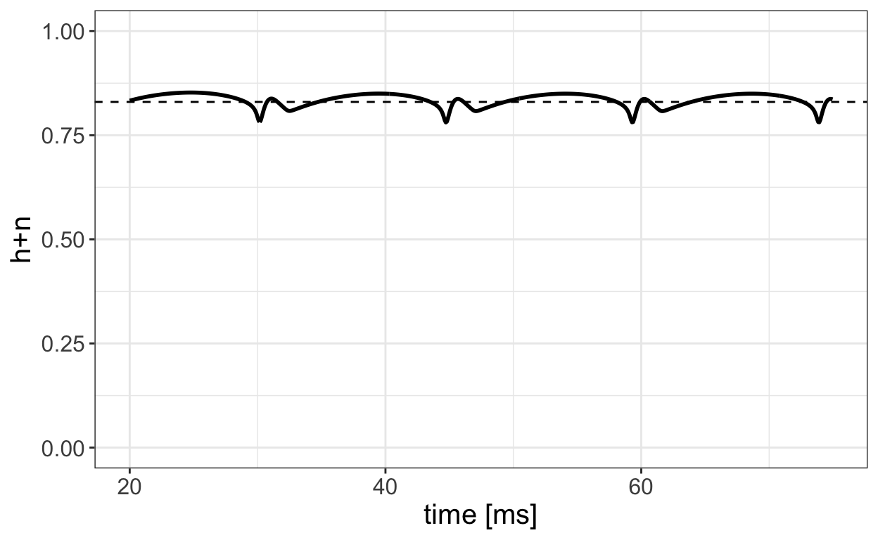
Further, let’s plot \(h(t) + n(t)\) as obtained from a numerical solution of the HH model for a range of time values.
Show code
# time points
t_initial <- 0
t_final <- 75
times <- seq(from = t_initial, to = t_final, by = 0.08)

# initial conditions
v0 <- -50
m0 <- alpha_m(v0)/(alpha_m(v0)+beta_m(v0))
yini <- c(v=v0, h=1, m=m0, n=0.4)

# numerical solution
out <- ode(y = yini, times = times, func = HH,
           parms = HH_parameters,method = "ode45")

HHsol <- data.frame(t=out[,"time"],v=out[,"v"],h=out[,"h"],m=out[,"m"],n=out[,"n"])

# plot
HHsol %>% mutate(h_plus_n=h+n) %>% filter(t >= 20) %>%
  ggplot(aes(x=t,y=h_plus_n)) + geom_line(lwd=1) +
  geom_hline(yintercept=0.83,linetype="dashed") + ylim(c(0,1)) +
  labs(x="time [ms]",y = "h+n") +
  theme_bw() + theme(text=element_text(size=15))

We observe that \(h(t) + n(t) \approx 0.83\) for much of the time. Based on this observation, we set \(h + n = 0.83\) which gives \(h = 0.83 - n\) allowing for the elimination of the \(h\) equation from the classical HH model.
Two-Dimensional Reduced HH
Making the two simplifications previously described reduces the Hodgkin-Huxley model to a two-dimensional system
\[ \begin{align} C\frac{dv}{dt} &= \bar{g}_{\text{Na}}m_{\infty}(v)^3 (0.83 - n)(v_{\text{Na}} - v) + \bar{g}_{\text{K}}n^4(v_{\text{K}} - v) + \bar{g}_{\text{L}}(v_{\text{L}} - v) + I \\ \frac{dn}{dt} &= \frac{n_{\infty}(v) - n}{\tau_{n}(v)} \end{align} \]
We call this system the two-dimensional reduced Hodgkin-Huxley model. This system has the form
\[ \begin{align} \frac{dv}{dt} &= f(v,n) \\ \frac{dn}{dt} &= g(v,n) \end{align} \]
which is a two-dimensional nonlinear autonomous system and thus can be studied via phase-plane methods.
Nullclines for Reduced HH
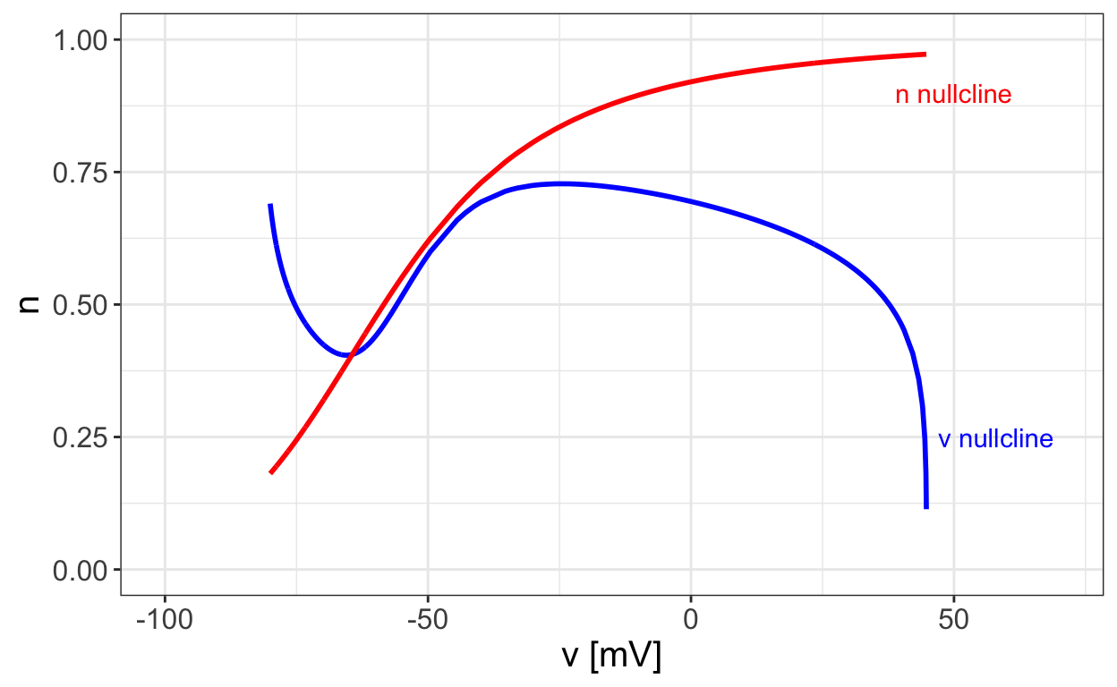
The first step in a phase-plane analysis of the two-dimensional reduced Hodgkin-Huxley model is to examine the nullclines for the system. These are shown in the next figure.
Show code
# initial conditions
yini <- c(v=-55, n=0.0)

# numerical solution
out <- ode(y = yini, times = times, func = HH_reduced,
           parms = HH_parameters,method = "ode45")

HHsol_reduced <- data.frame(t=out[,"time"],v=out[,"v"],n=out[,"n"])

v_nulls <- map_dbl(HHsol_reduced$v,compute_v_null)
n_nulls <- n_inf(HHsol_reduced$v)

HHsol_reduced <- HHsol_reduced %>% mutate(v_nulls=v_nulls,n_nulls=n_nulls)

ggplot(HHsol_reduced) + geom_line(aes(x=v,y=v_nulls),color="blue",lwd=1) +
  annotate(geom="text", x=58, y=0.25, label="v nullcline",
              color="blue") +
  geom_line(aes(x=v,y=n_nulls),color="red",lwd=1) +
    annotate(geom="text", x=50, y=0.9, label="n nullcline",
              color="red") +
  xlim(c(-100,70)) + ylim(c(0,1)) +
  xlab("v [mV]") + ylab("n") +
  theme_bw() + theme(text=element_text(size=15))

Note that in order to determine the \(v\) nullcline we need to solve the nonlinear equation
\(\bar{g}_{\text{Na}}m_{\infty}(v)^3 (0.83 - n)(v_{\text{Na}} - v) + \bar{g}_{\text{K}}n^4(v_{\text{K}} - v) + \bar{g}_{\text{L}}(v_{\text{L}} - v) + I = 0\)
for \(n\) in terms of \(v\). It is not possible to do this easily
in closed form so we utilize a root-finding algorithm via the
uniroot function in order to do this numerically.
Notice that there is a unique equilibrium point where the two nullclines intersect. Furthermore, one nullcline is monotonically increasing while the other has one local minimum and one local maximum. These are important geometric features that we will return to later on.
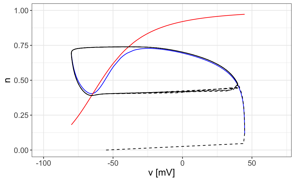
The next plot shows the nullclines together with a trajecory that approaches a limit cycle.
Show code

Notice how the trajectory “flows along” part of the one nullcline. Let’s examine how this corresponds to the time series plot of the solution.
Slow-Fast Dynamics
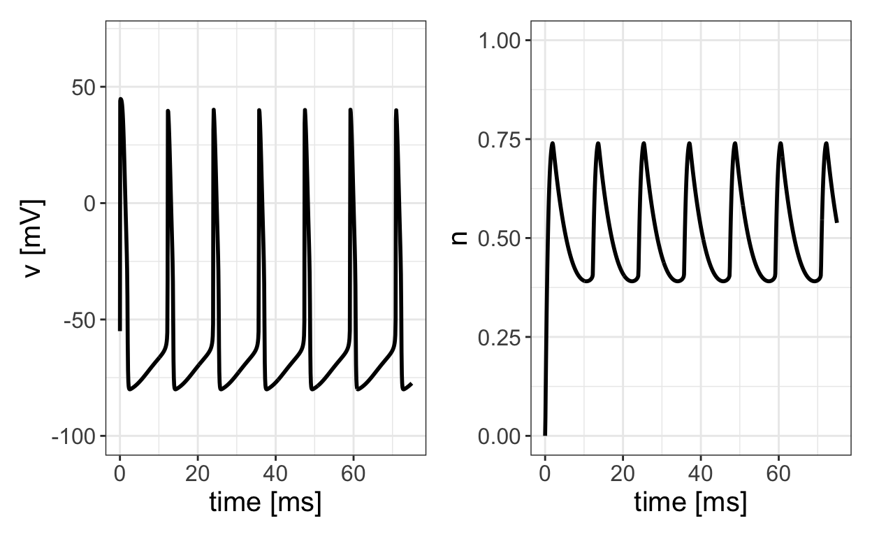
The following figure displays the potential \(v\) and gating variable \(n\) as a functions of time corresponding to the trajectory in the previous phase-plane plot.
Show code
p1 <- ggplot(HHsol_reduced) + geom_line(aes(x=t,y=v),lwd=1) +
  ylim(c(-100,70)) +
  xlab("time [ms]") + ylab("v [mV]") +
  theme_bw() + theme(text=element_text(size=15))
p2 <- ggplot(HHsol_reduced) + geom_line(aes(x=t,y=n),lwd=1) +
  ylim(c(0,1)) +
  xlab("time [ms]") + ylab("n") +
  theme_bw() + theme(text=element_text(size=15))

p1 + p2

We see that there are two time-scales at play here. There is a slow time-scale corresponding to the time it takes the potential to increase up to the firing threshold, and then there is a fast time-scale associated with the quick spike in potential. This means that the speed of a trajectory around the limit cycle is not constant. The motion is slow along the left side of the limit cycle corresponding to the slow increase in potential from its minimum value to the firing threshold value. During this time, there is a slow decrease in the value of \(n\). The right hand side of the limit cycle corresponds to the fast increase and decrease in \(v\) associated with the action potential spike. This type of two-time-scale dynamics is called slow-fast dynamics. One often refers to \(n\) as the slow variable and \(v\) as the fast variable. Oscillations associated with slow-fast dynamics such as we see with the reduced HH model are called relaxation oscillations. As we will see, the analysis of slow-fast dynamics and relaxation oscillations is a major theme in mathematical/computational studies of neural and cardiac systems. In fact, mathematical methods such as geometric singular perturbation theory have been developed in part to study such dynamics.
While the two-dimensional reduced Hodgkin-Huxley model is obtained by direct simplification of the classical HH ODEs, it is also possible to obtain systems with dynamics similar to that of the reduced HH model by a sort of geometric simplification.
The FitzHugh-Nagumo Model
Recall that for the two-dimensional reduced Hodgkin-Huxley model, one nullcline is monotonically increasing while the other has one local minimum and one local maximum. Now, a straight line is monotonically increasing and a cubic polynomial has one local minimum and one local maximum. So, what if we replace the \(n\) nullcline with a straight line and the \(v\) nullcline with a cubic? The following system, known as the FitzHugh-Nagumo model (FH) does exactly that.
\[ \begin{align} \frac{dv}{dt} &= v - \frac{v^3}{3} - n + I\\ \frac{dn}{dt} &= \frac{av - n}{\tau_{n}} \end{align} \]
We leave it as an exercise to show that the FitzHugh-Nagumo model exhibits slow-fast relaxation oscillations similar to those of the reduced HH model.
Note that the HH, reduced HH, and FH models all have a parameter \(I\) for input current. In some cases, this may act as a bifurcation parameter. This is the topic we take up in the next section of notes.
Further Reading
Our discussion largely follows Chapter 10 from (Börgers 2017). The texts (Ermentrout and Terman 2010) and (Gerstner et al. 2014) provides similar coverage but goes further into some of the mathematics associated with mathematical neuroscience. You can access (Gerstner et al. 2014) for free online here.