Course Notes 14

An introduction to linear difference equations.

Goals

After reading this section of notes, you should

1. know what is a discrete-time model,

2. know what is a linear difference equation,

3. know how to use linear algebra techniques to analyze a linear difference equation, and

4. be aware of some biomathematical applications of linear difference equations.

Background

Let N(t) denote the number of a single isolated and homogeneous population at time t. A common question is how does the population change over time? Early on, we argued that a general model for this is

N(t+Δt)=N(t)+G(N(t),Δt)

which essentially states that the change (increase or decrease) in the population from t to t+Δt is determined by the current population N(t) incremented by some “growth” function G(N(t),Δt) which could be positive or negative. A first order approximation for G is

G(N(t),Δt)=rΔtN(t)

where we do not make any assumptions about the sign of r. This leads to

N(t+Δt)=N(t)+rΔtN(t)

Previously, we rewrote the last expression as

N(t+Δt)−N(t)Δt=rN(t)

and took the limit as Δt→0 which lead to the exponential growth model dNdt=rN. This involves making an assumption. Specifically, we assume that time t can be reasonably treated as a continuous variable. There are many situations where this an appropriate assumption. On the other hand, there are situations in which it is more reasonable to view time as a discrete variable. Let’s now make this assumption in the context of our population growth model. To denote this distinction mathematically, we write N(t)=Nt, then our simple first-order population growth model becomes

Nt+Δt=(1+rΔt)Nt

If we increment over a fixed-size time step for Δt, then we can write the previous equation as

Nt+1=λNt

This is an example of a discrete time model. In general, a discrete time model is a sequence x0, x1, …, xn, xn+1, …, where

xi∈Rp for all i=0,1,… and for some p∈Z+, and

xi+1=f(xi,xi−1,xi−2,…,xi−k) for all i=1,2,… and some fixed k≥0.

Typically, we treat the xi as unknowns and refer to the expression xi+1=f(xi,xi−1,xi−2,…,xi−k) as a difference equation. A solution of the difference equation is any sequence x0,x1,… that satisfies the recurrence defined by the difference equation.

If k=0, then we have

xi+1=f(xi)

and the discrete time model is said to be first-order.

In our example model Nt+1=λNt we have f(Nt)=λNt with λ a constant. It is obviously a first-order model. Moreover, it is linear. In general, if a discrete time model can be written as

xt+1=Axt

where xt∈Rn for all t and A is an n×n matrix then we say it is a linear difference equation.

Analysis of Linear Difference Equations

Suppose we have a linear difference equation

xt+1=Axt

where xt∈Rn for all t and A is an n×n matrix, and let x0 be some given initial vector. Then,

x1=Ax0,x2=Ax1=A(Ax0)=A2x0,

and generally,

xi+1=Axi=A(Axi−1)=A2xi−1=A(A(Axi−2))=A3xi−2=…=Ak+1xi−k=…=Ai+1x0

Thus, the solution to a linear difference equation xt+1=Axt is a sequence x0, x1=Ax0, x2=A2x0, …, xn=Anx0, …. Notice that to compute each term in the sequence, we must compute the n-fold matrix power An. Typically, this is not convenient to compute. Our goal is to show that there is another approach that can be taken.

Eigenvalue Analysis of Linear Difference Equations

Let A be an n×n matrix and suppose that A has a complete set of eigenvectors. That is, suppose that A has n linearly independent eigenvectors v1,v2,…,vn with corresponding eigenvalues λ1,λ2…,λn. Now, let x0 be a vector in Rn. We may write

x0=c1v1+c2v2+⋯+cnvn

where the ci are uniquely determined scalars. Further, if λ, v is an eigenvalue-eigenvector pair for A, then

Anv=λnv,

an identity you may derive as an exercise. Using this, we see that

xi=Aix0=c1λi1v1+c2λi2v2+⋯+cnλinvn

and this provides another way to express a solution to a linear difference equation. The benefit is that this does not require us to compute matrix powers, only powers of scalars.

Example

Consider the linear difference equation xt+1=Axt with

A=(2321),

the eigenvalues of A are

Show code

A <- matrix(c(2,3,2,1),2,2,byrow=TRUE)
eigen(A)$values

[1]  4 -1

One can also see that if λ1=4 and λ2=−1, then v1=(3,2)T and v2=(1,−1)T are corresponding eigenvectors. Thus, the general solution to this example linear difference equation is

xi=c1(4)i(32)+c2(−1)i(1−1)

Suppose for example that x0=(1,1)T. To find the solution with this particular initial condition we must find scalars c1 and c2 so that

(11)=c1(32)+c2(1−1)

this can be done by solving the linear system

(312−1)(c1c2)=(11)

which is

Show code

V <- matrix(c(3,1,2,-1),2,2,byrow = TRUE)
b <- c(1,1)
(x<-solve(V,b))

[1]  0.4 -0.2

So, the solution to xt+1=Axt with

A=(2321),

and x0=(1,1)T is

xt=25(4)t(32)−15(−1)t(1−1)=(4)t(6545)+(−1)t(−1515)

An interesting question about the dynamics of discrete time models is, what happens to the system as t→∞. Note that in the expression

xi=c1λi1v1+c2λi2v2+⋯+cnλinvn

if all of the eigenvalues satisfy |λi|<1, then xi→0 as i→∞. Thus, if xt+1=Axt is a linear difference equation, we expect xt→0 in the long-term whenever all of the eigenvalues of A have absolute value less than 1.

We can apply the result we just derived to our simple population growth model Nt+1=λNt by observing that it is a one-dimensional linear difference equation. Therefore, the general solution is Nt=cλtN0 and then the population will die out if |λ|<1. On the other hand, what will happen if |λ|>1? In the one-dimensional case it is pretty clear, the magnitude of the population will grow without bound. What happens in the general case xt+1=Axt whenever A is an n×n matrix?

To answer this question, suppose that our eigenvalues are ordered so that |λ1|>|λ2|>⋯>|λn| and then rewrite

xt=c1(λ1)tv1+c2(λ2)tv2+⋯+cn(λn)tvn=λt1(c1v1+c2(λ2λ1)tv2+⋯+cn(λnλ1)tvn)

Now, for j=2,…n we have that |λjλ1|<1. So, we expect that as t→∞ each of these terms will go to zero and xt will asymptotically approach the line determined by the vector v1. For a matrix A, we call the eigenvalue of A that is largest in absolute value the dominant eigenvalue. Thus, the dominant eigenvalue and corresponding eigenvector determine the long-term dynamics of a discrete dynamical system determined by a linear difference equation.

Example

Consider again the linear difference equation xt+1=Axt with

A=(2321)

This matrix has dominant eigenvalue λ1=4 with corresponding eigenvector v1=(3,2)T. The following figure shows the points xt in the plane determined by the sequence xt=Atx0 together with the line through the vector v1.

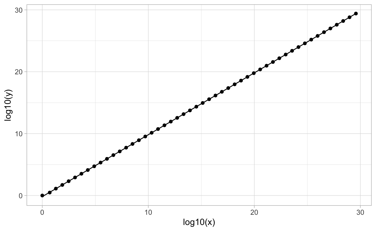
Note that we have plotted on the log scale because there is exponential growth in the magnitude of points in the sequence of vectors xt. This plot clearly shows how the asymptotic dynamics of the discrete time model “follows” the direction of the eigenvector corresponding with the dominant eigenvalue.

Note: Of course it may be the case that a particular n×n matrix A does not have n distinct eigenvalues. In such cases it is still possible to analyze the linear difference equation xt+1=Axt but the linear algebra becomes slightly more complicated. We leave such a discussion to one of the references such as (Allen 2007) or (de Vries et al. 2006).

Application: Age-Structured Models

An important application of linear difference equations as a discrete time model for population growth is provided by the so-called Leslie matrix model. The utility of this model is that it allows us to incorporate additional biologically interesting structure into a population model. By “structure” we mean a feature or features that subsets of a population may or may not have but that plays a distinguishing role in the ecology of the species whose population growth we want to model.

For example, many insects progress through distinct, discrete developmental stages such as egg, larva, pupa, adult. The reproductive behavior and survival rate is different within each of these different developmental stages. Thus, there is a clear age-structure involved in the growth of such species. How does one incorporate such additional structure into a mathematical model for the growth of a population? It is clear that age is a temporal phenomenon but aging may occur on a different time-scale than the overall change in the size of a population. This makes it challenging to incorporate age-structure into a continuous-time model although this can be done using partial differential equations. On the other hand, it is fairly simple to develop discrete time models that include age-structure or other similar population structures. This is done classically using the Leslie matrix model.

Here is the general idea. To start with the simplest case we assume that we have a single population that is closed to migration and we only model females. The population is divided up into discrete groups, say for example into N groups. Denote by (xi)t the number of individuals in group i at time t. We assume that group 1 corresponds to new offspring. Thus, new individuals are “born into” group 1. For each of the groups i=1,2,…,N, there is a chance of progressing from group i to group i+1 determined by a value si. Further, for i=1,2,…,N we let bi≥0 denote the average number of newborn females produced by one female in the i-th age group that survive through the time interval in which they were born. Then,

(x1)t+1=b1(x1)t+b2(x2)t+⋯+bN(xN)t

(xi+1)t+1=si(xi)t, for i=1,…,N−1

We can rewrite this in matrix-vector notation as

Xt+1=((x1)t+1(x2)t+1(x3)t+1⋮(xN)t+1)=(b1b2⋯bN−1bNs10⋯000s2⋯00⋮⋮⋱⋮⋮00⋯sN−10)((x1)t(x2)t(x3)t⋮(xN)t)=LXt

where we call the matrix L the Leslie matrix. Here is a diagram that illustrates the Leslie matrix model idea in the case where N=4:

Show code

a_graph <-
  create_graph() %>%
  add_n_nodes(n=4,label = c("1","2","3","4"),
              node_aes = node_aes(shape="circle",color = "black")) %>%
  add_edges_w_string(edges = "1->2 2->3 3->4 4->1 3->1 2->1 1->1") %>%
  select_edges_by_edge_id(edges = 1:7) %>%
  set_edge_attrs_ws(
    edge_attr = color,
    value = "black")


render_graph(a_graph, layout = "circle")

This diagram shows the relationships among the (four in the example) different age groups.

Before we proceed to consider the analysis of the dynamics of a Leslie matrix model, note that for any Leslie matrix L, all of the entries will be nonnegative.

Analyzing the Leslie Matrix Model

Given an n×n Leslie matrix L, a typical problem is to determine if its coefficients are such that L has a strictly dominant eigenvalue λ1. That is, a unique eigenvalue λ1 such that |λ1|>|λj| for j=2,3,…,n. As we have seen in a previous section, if this is the case then λ1 and its corresponding eigenvector v1 determine the long-term dynamics of the Leslie model. In the context of Leslie models, an eigenvector v1 associated with a strictly dominant eigenvalue λ1 is called a stable age distribution.

We suspect from our previous analysis of linear difference equations that if λ1 is a strictly dominant eigenvalue, then

• if |λ1|<1, then the overall population size will decrease over time, and

• if |λ1|>1, then the population increases over time in the direction of the stable age distribution v1.

Note that if L is a Leslie matrix with a strictly dominant eigenvalue λ1, then the entries of the stable age distribution v1 will be positive.

Much theory has been developed for a general analysis of Leslie matrix models, see section 1.7 of (Allen 2007) for the details. Here we will simply consider some examples.

Example 1

Suppose that we have a population with two age groups where only one of the two ages is reproducing. Then the Leslie matrix model has

L=(0b2s10)

where b2 and s1 are positive real values. The eigenvalues for this L are obtained by solving the quadratic polynomial

λ2−0λ+(−b2s1)=0

and thus are λ1,2=±√b2s1

In this case, there is no strictly dominant eigenvalue because |λ1,2|=√b2s1 and there is not a unique eigenvalue with the largest magnitude.

Example 2

Suppose that we have a population with two age groups where both are reproducing. Then the Leslie matrix model has

L=(b1b2s10)

where b1, b2, and s1 are positive real values. The eigenvalues for this L are obtained by solving the quadratic polynomial

λ2−b1λ+(−b2s1)=0

and thus are

λ1,2=b1±√b21+4b2s12

Thus, there is a strictly dominant eigenvalue λ1=b1+√b21+4b2s12 and we have that λ1>0. Furthermore,

λ1=b1+√b21+4b2s12>b1+√b212=b1

from which we see that if b1>1, then λ1>1. Note however that this is not the only situation in which we can have λ1>1.

Let’s find the eigenvector v1 corresponding to λ1=b1+√b21+4b2s12. Such a vector will satisfy

(L−λ1I)v1=(b1−√b21+4b2s12b2s1−b1−√b21+4b2s12)(xy)=(00)

and you can show (for homework) that

v1=(1s1λ1)=(12s1b1+√b21+4b2s1)

satisfies the above equation. Thus,

L=(b1b2s10)

has strictly dominant eigenvalue λ1=b1+√b21+4b2s12 with stable age distribution

v1=(1s1λ1)=(12s1b1+√b21+4b2s1)

Example 3

Consider the following three-stage Leslie matrix

L=(091213000120)

We can compute the eigenvalues and eigenvectors for L with R:

Show code

L <- matrix(c(0,9,12,1/3,0,0,0,1/2,0),3,3,byrow = TRUE)
(Ls <- eigen(L))

eigen() decomposition
$values
[1]  2+0i -1+0i -1-0i

$vectors
               [,1]          [,2]          [,3]
[1,] -0.98556187+0i  0.9370426+0i  0.9370426+0i
[2,] -0.16426031+0i -0.3123475-0i -0.3123475+0i
[3,] -0.04106508+0i  0.1561738+0i  0.1561738-0i

From this, we see that L has a strictly dominant eigenvalue λ1=2 with corresponding stable stage distribution -0.985561874823818+0i, -0.164260312470636+0i, -0.0410650781176591+0i. Let’s simulate the dynamics of Xt+1=LXt for many times-steps and compare the last values with v1:

Show code

N <- 100
x <- c(10,5,2)
for (i in 1:N){
  x <- L %*% x
}
x

             [,1]
[1,] 2.929681e+31
[2,] 4.882802e+30
[3,] 1.220701e+30

We see that the population grows over time. Do the population values grow in the direction of v1? In order to determine this, we can determine the distance between our last iterate and the line through v1, or equivalently, we can compute the angle between the two vectors.

[1] 3.141593+0i

If the angle between two vectors is 0 or π then they lie on the same line. We see that our two vectros are essentially parallel. We can confirm this by normalizing each of the vectors:

[1] -0.98556187+0i -0.16426031+0i -0.04106508+0i

           [,1]
[1,] 0.98556187
[2,] 0.16426031
[3,] 0.04106508

These vectors are obviously nearly parallel. More examples and problems related to Leslie matrix models will be considered in the homework exercises.

Conclusion

We’ve introduced linear difference equations as an example of discrete time systems and derived the role that the eigenvalues and eigenvectors play in analyzing the dynamics of such systems. Notice that much of this analysis closely parallels the analysis of continuous-time linear autonomous systems. An important example of linear difference equations in biomathematics is the Leslie matrix model approach to representing the population dynamics for a structured population. Next, we will study another class of discrete time systems by looking at first-order nonlinear difference equations. As we will see, even very simple nonlinear difference equations can exhibit very complex dynamics.

Further Reading

For more on discrete time models and linear difference equations in particular, see chapter 1 from either (Allen 2007) or (de Vries et al. 2006). Both of these books also contain references to further reading on the topics of difference equations and their applications within biomathematics.An excellent general reference for structured population models is (Cushing 1998).