Course Notes 17

Ruling out closed orbits.

Goals

After reading this section of notes, you should

1. know what a gradient system is and understand why such a system can not have a closed orbit,

2. know what a Liapunov function is, and

3. know Dulac’s criterion and how to apply it.

Background

From our experiences so far, we know that a two-dimensional autonomous system of the form

\[ \begin{align} \frac{dx}{dt} &= f(x,y) \\ \frac{dy}{dt} &= g(x,y) \end{align} \] may possess closed orbits either in the form of a nonlinear center or a limit cycle. However, in general, it is tricky to confirm the existence of a closed orbit for a nonlinear system. In this section of notes, we provide some techniques for ruling out the possibility of closed orbits. Here we closely follow section 7.2 from (Strogatz 2015) and recommend it for further reading.

Techniques for Ruling Out Closed Orbits

In this section, we introduce three common and relatively easy techniques that can be used to rule out the possibility that a system of the form

\[ \begin{align} \frac{dx}{dt} &= f(x,y) \\ \frac{dy}{dt} &= g(x,y) \end{align} \]

possesses closed orbits. These are gradient systems, Liapunoz functions, and Dulac’s criterion.

Gradient systems

Suppose that \(F:\mathbb{R}^{n} \rightarrow \mathbb{R}\) is a function such that \(\frac{\partial F}{\partial x_{i}}\) exists for \(i=1,2,\ldots , n\). We define the gradient \(\nabla F\) of \(F\) to be the vector

\[ \nabla F(x_{1},x_{2},\ldots, x_{n}) = \left(\begin{array}{c} \frac{\partial F}{\partial x_{1}}(x_{1},x_{2},\ldots, x_{n}) \\\frac{\partial F}{\partial x_{2}}(x_{1},x_{2},\ldots, x_{n}) \\ \vdots \\ \frac{\partial F}{\partial x_{n}}(x_{1},x_{2},\ldots, x_{n}) \end{array}\right) \]

In particular, in two-dimensions

\[ \nabla F(x,y) = \left(\begin{array}{c} \frac{\partial F}{\partial x}(x,y) \\ \frac{\partial F}{\partial y}(x,y) \end{array}\right) \]

Notation: We will use bold face letters such as \({\bf x}\) to stand for vectors. That is, \({\bf x} = (x_{1},x_{2},\ldots , x_{n})^{T}\). Further, notation such as \({\bf f}({\bf x})\) denotes concisely a vector field such as

\[ {\bf f}({\bf x}) = \left(\begin{array}{c} f_{1}(x_{1},x_{2},\ldots, x_{n}) \\ f_{2}(x_{1},x_{2},\ldots, x_{n}) \\ \vdots \\ f_{n}(x_{1},x_{2},\ldots, x_{n}) \end{array}\right) \]

Definition: Gradient system

We say that a system \(\frac{d}{dt}{\bf x}={\bf f}({\bf x})\) is a gradient system if there is a (scalar) function \(F({\bf x})\) that satisfies \(-\nabla F = {\bf f}({\bf x})\) in which case we have \(\frac{d}{dt}{\bf x} = -\nabla F\). Sometimes a gradient system is also called a conservative system and the function \(F\) is called a potential.

In the plane \(\mathbb{R}^2\), a system

\[ \begin{align} \frac{dx}{dt} &= f(x,y) \\ \frac{dy}{dt} &= g(x,y) \end{align} \]

is a gradient system if there is a function \(F(x,y)\) satisfying

\[ \begin{align} \frac{dx}{dt} &= f(x,y) = -\frac{\partial F}{\partial x} \\ \frac{dy}{dt} &= g(x,y) = -\frac{\partial F}{\partial y} \end{align} \]

For example, the system

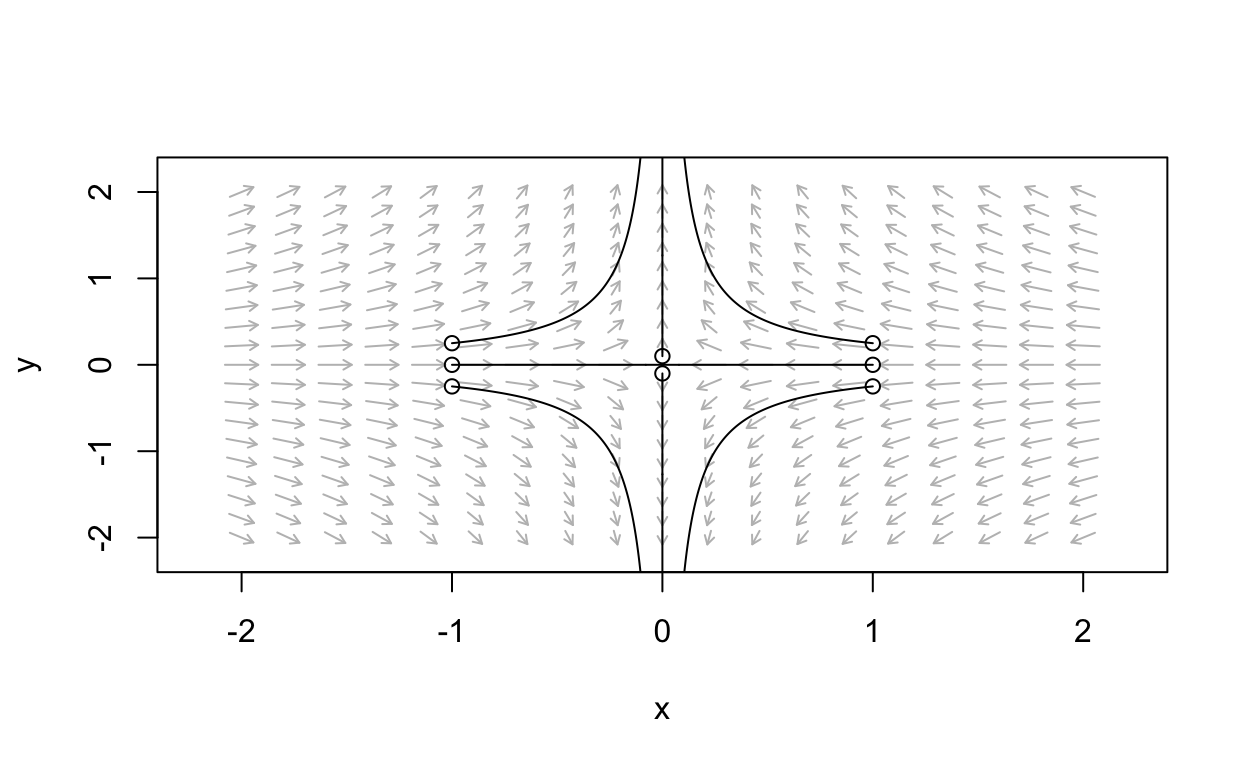
\[ \begin{align} \frac{dx}{dt} &= -2x\\ \frac{dy}{dt} &= 2y \end{align} \] is a gradient system with potential \(F(x,y) = x^2 - y^2\) since

\[ \begin{align} -\frac{\partial F}{\partial x} &= -2x\\ -\frac{\partial F}{\partial y} &= -(-2y) = 2y \end{align} \] Now this particular system happens to be linear with trace \(\tau = 0\) and determinant \(\delta = -4\) from which we deduce that the origin is a saddle. The phase portrait for the system is shown below.

Show code

lin_sys <- function(t,state,parameters){
  with(as.list(c(state,parameters)),{
    
    dx <- A %*% state
    
    list(dx)
  })
}

A <- matrix(c(-2,0,0,2),2,2,byrow=TRUE)

parms_mat <- list(A=A)
linear_flowField  <- flowField(lin_sys,
                                       xlim       = c(-2, 2),
                                       ylim       = c(-2, 2),
                                       parameters = parms_mat,
                                       points     = 19,
                                       add = FALSE)
state                        <- matrix(c(1,0,1.0,0.25,-1.0,0.25,-1.0,-0.25,1.0,-0.25,-1,0,0,0.1,0,-0.1),
                                    8, 2, byrow = TRUE)
linear_trajectory <- trajectory(lin_sys,
                                        y0         = state,
                                        tlim       = c(0, 10),
                                        parameters = parms_mat,
                                        add=TRUE)

In general, gradient systems will not be linear. Further, not all linear systems are gradient systems.

Gradient systems and closed orbits

Theorem: Closed orbits are impossible in gradient systems.

See (Strogatz 2015) for a proof.

Given a system

\[ \begin{align} \frac{dx}{dt} &= f(x,y) \\ \frac{dy}{dt} &= g(x,y) \end{align} \] it may not be easy to find a potential function \(F\) even if the system is actually a gradient system. There is an approach that sometimes works. Let’s look at the example system

\[ \begin{align} \frac{dx}{dt} &= -2x\\ \frac{dy}{dt} &= 2y \end{align} \]

again. A potential \(F\) must satisfy \(\frac{\partial F}{\partial x}=-(-2x)=2x\). So let’s integrate this with respect to \(x\). Doing so gives

\(F(x,y) = \int 2x \ dx = x^2 + \phi(y)\)

Why do we have the additive term of \(\phi(y)\)? It is because any function of \(y\) alone is treated as a constant whenever we take a partial derivative with respect to \(x\). Now, if \(F(x,y) = x^2 + \phi(y)\) is actually a potential, then it must also satisfy

\[ \frac{\partial F}{\partial y} = \frac{\partial}{\partial y}(x^2 + \phi(y)) = \phi'(y) = -2y \] This happens provided \(\phi(y) = -y^2 + c\) for any constant value. This was obtained by integrating

\[ \int \phi'(y)\ dy = \int -2y \ dy \]

Thus, we conclude that \(F(x,y)=x^2 - y^2\) is a potential for the system

\[ \begin{align} \frac{dx}{dt} &= -2x\\ \frac{dy}{dt} &= 2y \end{align} \] Note that \(F(x,y)=x^2 - y^2 + c\) for any constant value of \(c\) would also be a potential for this system. Thus, potentials are only unique up to an additive constant.

In general, finding a potential in this way involes solving a system of differential equations

\[ \begin{align} \frac{\partial F}{\partial x} &= -f(x,y) \\ \frac{\partial F}{\partial y} &= -g(x,y) \end{align} \]

and this may or may not be easy depending on how difficult it is to find antiderivatives for the functions on the right hand side.

Contours of potential functions

Suppose that a system \[ \begin{align} \frac{dx}{dt} &= f(x,y)\\ \frac{dy}{dt} &= g(x,y) \end{align} \] is a gradient system with potential function \(F(x,y)\). As we know from Calculus III, the graph of \(z=F(x,y)\) is a surface but it can be visualized in the plane by displaying its contours. It turns out that the contours of a potential function \(F(x,y)\) are closely related to the phase portrait of the corresponding autonomous system.

In particular, a parametric curve \((x(t),y(t))\) that is a solution to a system

\[ \begin{align} \frac{dx}{dt} &= f(x,y)\\ \frac{dy}{dt} &= g(x,y) \end{align} \] that possesses a potential \(F(x,y)\) will be orthogonal to contour lines \(F(x,y)=c\). You will show that this is the case in the homework exercises.

For now, let’s make a contour plot of the potential \(F(x,y)=x^2-y^2\) for the system

\[ \begin{align} \frac{dx}{dt} &= -2x\\ \frac{dy}{dt} &= 2y \end{align} \]

the phase portrait of which was shown above.

Show code

F1 <- function(x) x[1]^2 - x[2]^2
cf_func(F1,xlim=c(-1.5,1.5),ylim=c(-1.5,1.5))

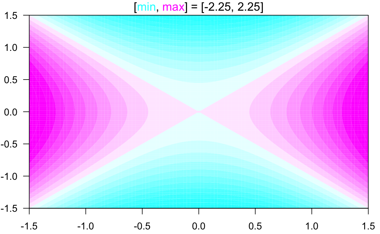
Can you see how the contour lines are orthogonal to the trajectories of the system? Note that we have used the function cf_func from the ContourFunctions package to obtain the previous plot.

Liapunov functions

Suppose that we have an autonomous system \(\frac{d}{dt}{\bf x}={\bf f}({\bf x})\) with an equilibrium \({\bf x}^{\ast}\). A function \(V\) that satisfies

1. \(V({\bf x}^{\ast})=0\) and \(V({\bf x}) > 0\) for all \({\bf x} \neq {\bf x}^{\ast}\), and

2. \(\frac{d}{dt}V({\bf x}) < 0\) for all \({\bf x} \neq {\bf x}^{\ast}\)

is called a Liapunov function.

Theorem: If a system \(\frac{d}{dt}{\bf x}={\bf f}({\bf x})\) with an equilibrium \({\bf x}^{\ast}\) has a Liapunov function, then the equilibrium \({\bf x}^{\ast}\) is globally asymptotically stable. Hence, the system cannot have a closed orbit.

That \({\bf x}^{\ast}\) is globally asymptotically stable means that for any initial condition \({\bf x}(t) \rightarrow {\bf x}^{\ast}\) as \(t\rightarrow \infty\). A system that has a globally asymptotically stable equilibrium cannot have a closed orbit since otherwise there would be at least one trajectory which would fail to approach the equilibrium \({\bf x}^{\ast}\). Thus, we can use the existence of a Liapunov function for the purpose of ruling out closed orbits.

Example

Consider the system

\[ \begin{align} \frac{dx}{dt} &= -x+4y \\ \frac{dy}{dt} &= -x - y^3 \end{align} \] We claim that \(V(x,y) = x^2 + 4y^2\) is a Liapunov function for this system. Note that the system has a single equilibrium at \({\bf x}^{\ast}=(0,0)\). Observe,

1. \(V(0,0)=0\) and \(V(x,y) > 0\) as long as \((x,y)\neq (0,0)\), and

\[ \begin{align} \frac{d}{dt}V(x,y) &= \frac{\partial V}{\partial x}\frac{dx}{dt} + \frac{\partial V}{\partial y}\frac{dy}{dt} \\ &= (2x)\frac{dx}{dt} + (8y)\frac{dy}{dt} \\ &= 2x(-x+4y) + 8y(-x - y^3) \\ &= -2x^2 + 8xy - 8xy - 8y^4 \\ &= -2x^2 - 8y^4 \end{align} \] for any trajectory of the system. Now, we have that \(-2x^2 - 8y^4 \leq 0\) and only equals zero at \((0,0)\). Thus \(V(x,y)=x^2 + 4y^2\) is in fact a Liapunov function for the system.

As you can check, the linearization of the system

\[ \begin{align} \frac{dx}{dt} &= -x+4y \\ \frac{dy}{dt} &= -x - y^3 \end{align} \]

at \((0,0)\) is

\[ \left(\begin{array}{cc} -1 & 4 \\ -1 & 0 \end{array}\right) \]

which has trace \(\tau = -1\) and determinant \(\delta = 4\). So we conclude that the phase portrait near \((0,0)\) is a stable spiral. The existence of a Liapunov function allows us to make an even stronger conclusion that the global phase portrait for the system is a stable spiral. We plot the phase portrait for this system here

Show code

nonlinear_example <- function(t,state,parameters){
  with(as.list(c(state,parameters)),{
    
    dx <- -state[1] + 4*state[2]
    dy <- -state[1] - state[2]^3
    
    list(c(dx,dy))
  })
}

nonlinear_flowfield  <- flowField(nonlinear_example,
                                       xlim       = c(-2, 2),
                                       ylim       = c(-2, 2),
                                       parameters = NULL,
                                       points     = 17,
                                       add = FALSE)

state <- matrix(c(1,1,-1,-1),2,2,byrow = TRUE)
nonlinear_trajs <- trajectory(nonlinear_example,
                                        y0         = state,
                                        tlim       = c(0, 10),
                                        parameters = NULL,add=TRUE)

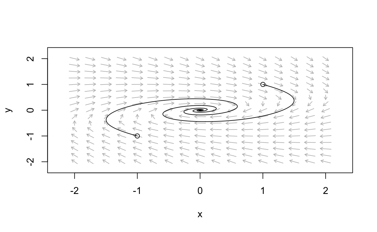
The stable spiral is apparent.

The method of Liapunov functions is very powerful. However, it is in general not trivial to find Liapunov functions.

Dulac’s criterion

The following result is known as Dulac’s criterion:

Theorem: Let \(\frac{d}{dt}{\bf x}={\bf f}({\bf x})\) be a continuously differentiable vector field defined on a simply connected region \(R\) of the plane \(\mathbb{R}^{2}\). If there exists a continuously differentiable, real-valued function \(s({\bf x})\) such that \(\nabla \cdot (s \frac{d}{dt}{\bf x})\) has one sign throughout \(R\), then there are no closed orbits lying entirely in \(R\).

Recall that the notation \(\nabla \cdot {\bf f}\) refers to the divergence of the vector field \({\bf f}\).

We refer to (Strogatz 2015) for the proof but note that the proof is an application of Green’s theorem from Calculus III.

Example

We use Dulac’s criterion to show that

\[ \begin{align} \frac{dx}{dt} &= y\\ \frac{dy}{dt} &= -x-y + x^2 + y^2 \end{align} \]

has no closed orbits. Obviously the right hand side of this system is a continuously differentiable vector field defined in the entire plane \(\mathbb{R}^2\) which happens to be a simply connected set (this essentially means that there are no holes in the plane). Now, let \(s(x,y)=e^{-2x}\), then

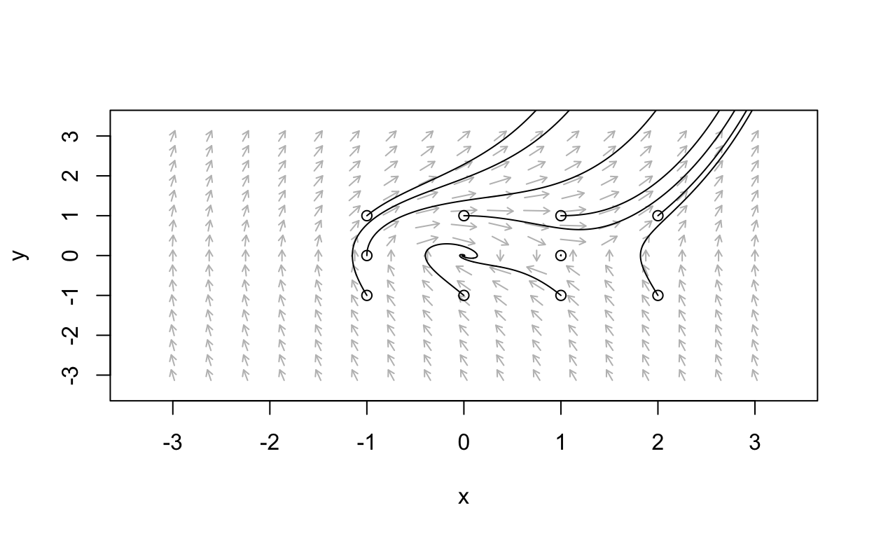
\[ \begin{align} \nabla \cdot (g(x,y) \left(\begin{array}{cc}\frac{dx}{dt} & \frac{dy}{dt} \end{array}\right)^{T}) &= \nabla \cdot (e^{-2x} \left(\begin{array}{cc}\frac{dx}{dt} & \frac{dy}{dt} \end{array}\right)^{T})\\ &= \frac{\partial }{\partial x}\left(e^{-2x}\frac{dx}{dt} \right) + \frac{\partial}{\partial y}\left(e^{-2x} \frac{dy}{dt} \right) \\ &= \frac{\partial }{\partial x}\left(e^{-2x}(y) \right) + \frac{\partial}{\partial y}\left(e^{-2x} (-x-y+x^2+y^2) \right) \\ &= -2ye^{-2x} - e^{-2x} + 2ye^{-2x} \\ &= -e^{-2x} < 0, \ \forall \ x \end{align} \] Thus, Dulac’s criterion is satisfied for this particular system. In the homework, you will be asked to determine the equilibria for the system

\[ \begin{align} \frac{dx}{dt} &= y\\ \frac{dy}{dt} &= -x-y + x^2 + y^2 \end{align} \]

and examine their corresponding stability properties. Further, you will rewrite the system in polar coordinates and see what that suggests about the phase portrait for the system which looks as follows

Show code

dulacs_example <- function(t,state,parameters){
  with(as.list(c(state,parameters)),{
    
    dx <- state[2]
    dy <- -state[1] - state[2] + state[1]^2 + state[2]^2
    
    list(c(dx,dy))
  })
}

nonlinear_flowfield  <- flowField(dulacs_example,
                                       xlim       = c(-3, 3),
                                       ylim       = c(-3, 3),
                                       parameters = NULL,
                                       points     = 17,
                                       add = FALSE)

state <- matrix(c(1,0,0,1,-1,0,0,-1,1,1,-1,1,-1,-1,1,-1,
                  2,-1,2,1),10,2,byrow = TRUE)
nonlinear_trajs <- trajectory(dulacs_example,
                                        y0         = state,
                                        tlim       = c(0, 50),
                                        parameters = NULL,add=TRUE)

Summary

Gradient systems, systems for which a Liapunov function exists, and systems for which Dulac’s criterion applies can not have closed orbits. This includes both limit cycles and nonlinear centers. If you have a system for which you have reason to believe that there should be no closed orbits, then you might be able to use one of these techniques to prove it. On the other hand, what do you do if you suspect that a system does possess closed orbits and you want to confirm it? In the case of stable limit cycles, the famous Poincarè-Bendixson theorem can often be used to provide a rigorous verification of the existence of a closed orbit. We will take up the study of this in the next section of notes.

Further Reading

For further details on the topics covered in this section of notes, see Chapter 7 from (Strogatz 2015).