Goals
After reading this section of notes, you should
know what is a first-order nonlinear difference equation,
know the procedure for determining fixed-points for first-order nonlinear difference equations, and
know how to use both graphical and analytical techniques for examining the stability properties of fixed-points for first-order nonlinear difference equations.
Introduction
Let’s return again to our general population model
\(N(t+\Delta t) = N(t) + G(N(t),\Delta t)\)
where \(N(t)\) denote the number of a single isolated and homogeneous population at time \(t\), and \(G(N(t),\Delta t)\) is a growth function which could be positive or negative. Further, let’s assume from the start that we are treating time as a discrete variable and therefore may write the model as
\(N_{t+1} = N_{t} + G(N_{t})\)
Previous, we took \(G\) to be a linear function of \(N_{t}\) and ended up with a model of the form \(N_{t+1}=\lambda N_{t}\). We noted that for \(N_{t+1}=\lambda N_{t}\) with \(\lambda > 1\) we obtain the discrete analog of exponential growth. As in the continuous time setting, exponential growth is unrealistic from an ecological perspective. Thus, we ask the question is there a nonlinear function \(G\) that may serve to “slow down” population growth as the population approaches a carrying capacity. One option is to take
\(G(N_{t}) = \rho (K - N_{t})N_{t}\)
You should take a moment to think about the properties of this particular \(G\) and how they relate to growth of the population. Now, with \(G(N_{t}) = \rho (C - N_{t})N_{t}\) we have
\(N_{t+1} = N_{t} + \rho (C - N_{t})N_{t}\)
This expression may be simplified as follows:
\[ \begin{align} N_{t+1} &= N_{t} + \rho (C - N_{t})N_{t} \\ & = N_{t} + \rho C N_{t} - \rho N_{t}^{2} \\ &= (1+\rho C) N_{t} - \rho N_{t}^{2} \\ &= (1+\rho C)\left(N_{t} - \frac{N_{t}^2}{\frac{1 + \rho C}{\rho}}\right) \\ &= (1+\rho C)N_{t}\left(1 - \frac{N_{t}}{\frac{1 + \rho C}{\rho}}\right) \\ &= rN_{t}\left(1 - \frac{N_{t}}{K} \right) \end{align} \]
where \(r= 1+\rho C\) and \(K= \frac{1 + \rho C}{\rho}\). Thus,
\(N_{t+1}=rN_{t}\left(1 - \frac{N_{t}}{K} \right)\)
is the discrete time logistic model. We can simplify this even further by non-dimensionalization. Let \(x_{t}=\frac{N_{t}}{K}\), then
\[ \begin{align} x_{t+1} &= \frac{N_{t+1}}{K} \\ &= \frac{1}{K}\left(rN_{t} \left(1 - \frac{N_{t}}{K} \right) \right) \\ &= rx_{t}(1-x_{t}) \end{align} \]
The non-dimensional discrete logistic model \(x_{t+1}=rx_{t}(1-x_{t})\) is an example of a first-order nonlinear difference equation. In general, first-order nonlinear difference equations take the form
\(x_{t+1} = f(x_{t})\)
where \(f\) is a nonlinear function. Moreover, first-order nonlinear difference equations provide another class of examples of discrete time systems.
There is already an important difference between the continuous logistic growth model
\(\frac{dN}{dt}=rN\left(1 - \frac{N}{K} \right)\)
and the discrete logistic growth model
\(N_{t+1} = rN_{t}\left(1 - \frac{N_{t}}{K} \right)\)
The continuous model non-dimensionalizes to \(\frac{dx}{dt}=x(1-x)\) while the discrete model non-dimensionalizes to \(x_{t+1}=rx_{t}(1-x_{t})\). In particular, we can not eliminate the parameter \(r\) from the discrete time model. Thus, we must be able to assess what are the dynamics of the discrete logistic model and how are they affected by the value of \(r\). We will see that \(x_{t+1}=rx_{t}(1-x_{t})\) possesses much richer dynamics than its continuous time counterpart.
Analyzing Nonlinear Difference Equations
Let \(x_{t+1}=f(x_{t})\) be a first-order nonlinear difference equation. We say that a value \(\xi\) is a fixed point for the system if it satisfies
\(\xi = f(\xi)\)
Note that a fixed point \(\xi\) for a difference equation \(x_{t+1}=f(x_{t})\) is a constant solution to the equation in a similar way as to how an equilibrium value is a constant solution to continuous autonomous system.
Given a difference equation \(x_{t+1}=f(x_{t})\), we can find its fixed points by solving the equation
\(x=f(x) \Leftrightarrow x-f(x) = 0\)
for the unknown \(x\).
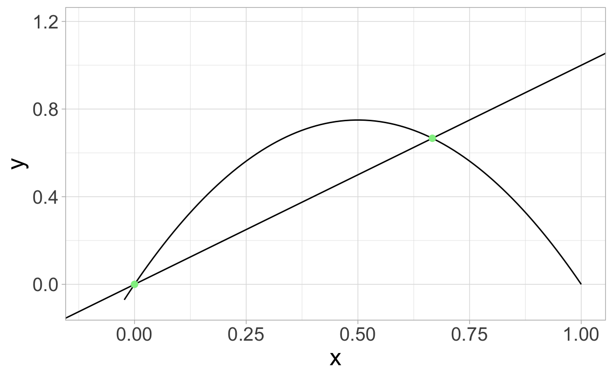
Graphically, fixed points for a difference equation \(x_{t+1}=f(x_{t})\) correspond ot points where the line \(y=x\) intersects the graph of \(y=f(x)\).
Example
Let’s determine the fixed points for the (non-dimensional) discrete logistic equation \(x_{t+1}=rx_{t}(1-x_{t})\). In order to do this, we must solve
\(x=rx(1-x) \Leftrightarrow x-rx(1-x) = 0 \Leftrightarrow x(1-r+rx)=0\)
which has solutions \(x=0\) and \(x=\frac{r-1}{r}\). Note that the second fixed point is only biologically reasonable if \(r \geq 1\).
The following plot shows the intersection of \(y=x\) and \(y=rx(1-x)\) in the case where \(r=3\).
Show code
ggplot(data=tibble(x=c(-0.1,1)),aes(x=x)) +
    geom_function(fun=function(x) 3.0*x*(1-x)) +
    geom_abline(slope = 1.0,intercept=0.0) +
    geom_point(x=c(0,2/3),y=c(0,2/3),color="lightgreen",size=2) +
    ylim(c(-0.1,1.2)) +
    xlab("x") +
    theme_light() +
    theme(text = element_text(size = 18))

Fixed Point Stability
Suppose that \(\xi\) is a fixed point for the difference equation \(x_{t+1}=f(x_{t})\). We say that \(\xi\) is stable if whenever \(x_{0}\) is sufficiently close but not equal to \(\xi\) we have that the sequence determined by \(x_{t+t}=f(x_{t})\) converges to \(\xi\).
We will make use of the following fact which is analogous to linear stability analysis for continuous autonomous systems:
If \(|f'(\xi)| < 1\), then \(\xi\) is stable.
If \(|f'(\xi)| > 1\), then \(\xi\) is unstable.
If \(|f'(\xi)|=1\) then we can not draw any conclusions.
Example
Let’s apply the stated linear stability analysis for nonlinear difference equations to the discrete logistic model \(x_{t+1}=f(x_{t})=rx_{t}(1-x_{t})\). We have that \(f'(x)=r-2rx\) and thus
\(|f'(0)| = r\), and
\(|f'\left(\frac{r-1}{r}\right)|=\left|2-r \right|\).
From this, we can see that \(\xi=0\) is stable if \(r<1\) and unstable if \(r > 1\). Note that if \(r<1\), then \(\xi=\frac{r-1}{r}\) does not make sense biologically.
Now, whenever \(3 > r > 1\) we can see that \(\xi=\frac{r-1}{r}\) will be stable since then we will have \(|2-r| < 1\). Further, if \(r > 3\), then \(\xi=\frac{r-1}{r}\) will be unstable. In order to know what happens when \(r=1\) or \(r=3\) we will need to rely on graphical techniques.
Cobweb Diagrams
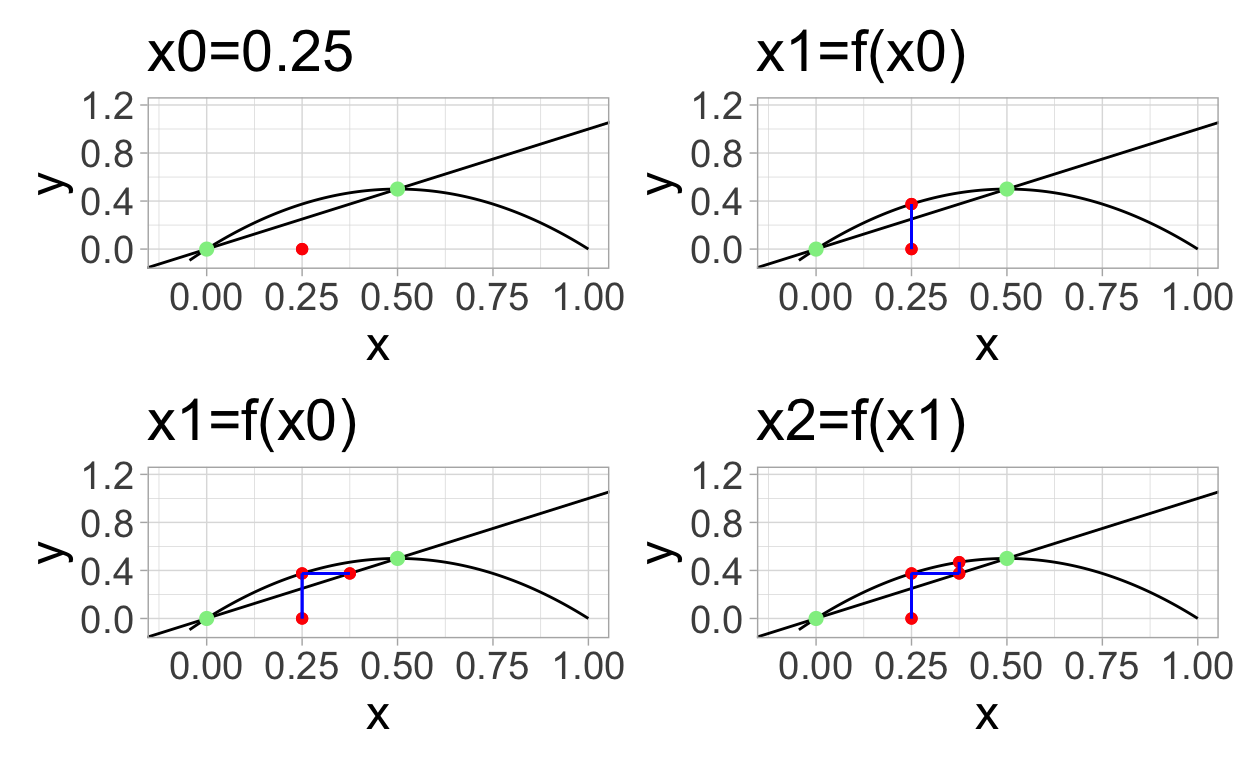
There is a graphical method for analyzing the dynamics and in particular the stability of first order nonlinear difference equations. This method is called cobwebbing and is carried out by constructing a so-called cobweb plot.
Suppose that we have a difference equation \(x_{t+1}=f(x_{t})\). We begin by plotting the graphs of \(y=x\) and \(y=f(x)\) on the same axes. This makes it possible to see the fixed points. Then, starting with an initial condition, \(x_{0}\), plot the series of points consecutively while connecting the points with a straight line at each step:
\[ \begin{align} &(x_{0},0) \\ &(x_{0},x_{1}=f(x_{0})) \\ &(x_{1},x_{1}) \\ &(x_{1},x_{2}=f(x_{1})) \\ &\ldots \\ &(x_{k},x_{k}) \\ &(x_{k},x_{k+1}=f(x_{k})) \\ & \text{so on} \end{align} \]
If the points \((x_{k},x_{k+1}=f(x_{k}))\) become increasingly close to \((\xi,\xi)\) then the fixed point is stable, otherwise the fixed point is unstable.
Here are the first four steps in creating a cobweb plot for \(x_{t+1}=2x_{t}(1-x_{t})\)
Show code
dl_2 <- function(x){2.0*x*(1-x)}

p1 <- ggplot(data=tibble(x=c(-0.1,1)),aes(x=x)) +
    geom_function(fun=dl_2) +
    geom_abline(slope = 1.0,intercept=0.0) +
    geom_point(x=c(0,1/2),y=c(0,1/2),color="lightgreen",size=2) +
    ylim(c(-0.1,1.2)) +
    xlab("x") +
    theme_light() +
    theme(text = element_text(size = 18))

x0 <- 0.25

p1 <- p1 +
    geom_point(x=x0,y=0.0,color="red") + ggtitle("x0=0.25")

x1 <- dl_2(x0)

p2 <- p1  + geom_point(x=x0,y=x1,color="red") +
  geom_segment(x=x0,y=0.0,
                     xend=x0,yend=x1,
                 color="blue") +
  ggtitle("x1=f(x0)")

p3 <- p2 + geom_point(x=x1,y=x1,color="red") +
  geom_segment(x=x0,y=x1,
               xend=x1,yend=x1,
               color="blue")

x2 <- dl_2(x1)

p4 <- p3 + geom_point(x=x1,y=x2,color="red") +
  geom_segment(x=x1,y=x1,
               xend=x1,yend=x2,
               color="blue") +
  ggtitle("x2=f(x1)")

(p1+p2) / (p3+p4)

Cobweb and Discrete Logistic Dynamics
To see and interact with the cobweb diagram for the discrete logistic model, check out this shiny web app. This app displays the time course for the dynamics of the discrete logistic model together with the corresponding cobweb plot.
To summarize the behavior of the discrete logistic model \(x_{t+1}=rx_{t}(1-x_{t})\), for values of the parameter \(r\):
If \(r<1\) then \(x=0\) is a stable fixed-point and the population decreases for any starting value \(0 < x_{0} < 1\).
If \(1 < r < 3\), then \(x=\frac{r-1}{r}\) is a stable fixed-point and the population tends toward the carrying capacity \(\frac{r-1}{r}\).
When \(r\) is around 3, the population oscillates in a periodic fashion.
If \(r\) is continuously increased up to 4 we see that the dynamics show a period doubling bifurcation and then eventually chaotic dynamics.
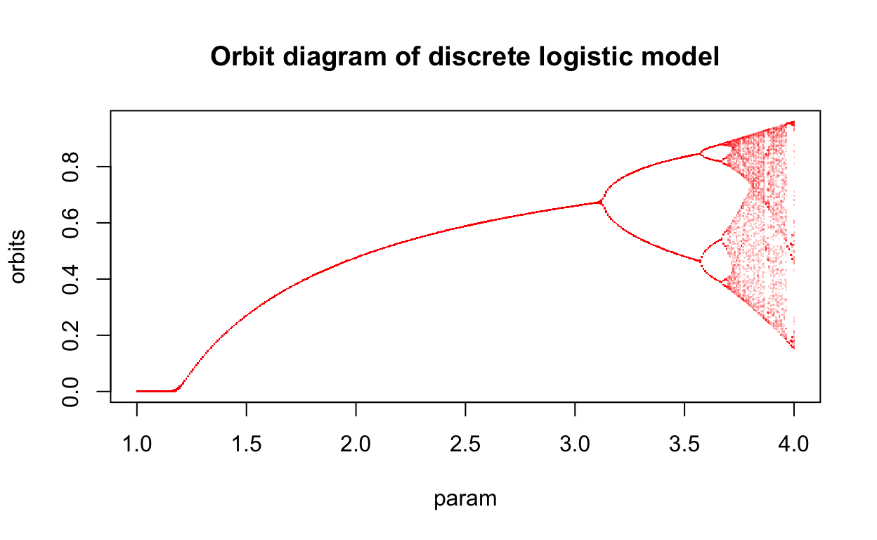
Thus, the dynamics of the discrete logistic model are very rich. We can summarize the changes in the dynamic behavior of the discrete logistic model using a so-called orbit diagram. Such a diagram shows the distinct values that an iteration \(x_{t+1}=f(x_{t})\) takes on (in the long-term) displayed vertically above values of a parameter such as \(r\) in the discrete logistic model. The following figure is the orbit diagam for \(x_{t+1}=rx_{t}(1-x_{t})\).
Show code
library(map1d)
plotOrbitDiagram(function(x, r) r * x*sin(1-x), 1, 4, 400, 200, 100)
title("Orbit diagram of discrete logistic model")

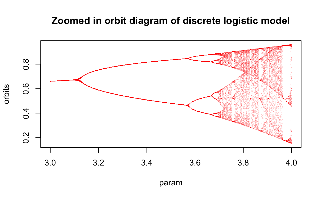
You can clearly see the period doubling behavior in this diagram. What is more, the diagram possesses self-similarity. That is, if we zoom in on a smaller portion of the diagram, we see all of the features of the larger diagram reproduced. Let’s zoom in a bit and take a closer look at what is happening after \(r\) gets to 3.
Show code
library(map1d)
plotOrbitDiagram(function(x, r) r * x*sin(1-x), 3, 4, 400, 200, 100)
title("Zoomed in orbit diagram of discrete logistic model")

Note that self-similarity is a hallmark feature of fractals. In fact, the orbit diagram for the discrete logistic model is an example of a fractal.
Further Reading
For more on discrete time models and linear difference equations in particular, see chapter 2 of (Allen 2007) or chapter 1 of (de Vries et al. 2006). Both of these books also contain references to further reading on the topics of difference equations and their applications within biomathematics. You can learn more about chaos and fractals as theses concepts relate to dynamical systems from (Strogatz 2015).