Course Notes 18

An introduction to the Poincarè-Bendixson theorem.

Goals

After reading this section of notes, you should

1. know what the Poincarè-Bendixson theorem says and understand how to use it to derive the existence of a stable limit cycle, when applicable.

Background

Consider the nonlinear autonomous two-dimensional system

dxdt=x(1−x2−y2)−y+μx2√x2+y2dydt=y(1−x2−y2)+x+μxy√x2+y2

Using the expression

drdt=1r(xdxdt+ydydt)dθdt=1r2(xdydt−ydxdt)

that we derived in our discussion on polar coordinates, one can rewrite the previous system as

drdt=r(1−r2)+μrcos(θ)dθdt=1

from which it is easy to see that whenever μ=0 the system has a stable limit cycle in the form of the circle r=1. The phase portrait for this system in the case μ=0 is shown below.

Show code

pb_example <- function(t,state,parameters){
  with(as.list(c(state,parameters)),{
    x <- state[1]
    y <- state[2]
    r <- sqrt(x^2+y^2)
    if (x==0.0 && y==0.0){
      dx <- 0.0
      dy <- 0.0
    }else{
    dx <- x*(1-x^2-y^2) - y + mu*x^2/r
    dy <- y*(1-x^2-y^2) + x + mu*x*y/r
    }
    
    list(c(dx,dy))
  })
}
nonlinear_flowfield  <- flowField(pb_example ,
                                       xlim       = c(-2, 2),
                                       ylim       = c(-2, 2),
                                       parameters = c(mu=0.0),
                                       points     = 17,
                                       add = FALSE)
state <- matrix(c(-0.25,0.25,1.0/sqrt(2.0),1.0/sqrt(2.0),0.0,2.0),3,2,byrow = TRUE)

nonlinear_trajs <- trajectory(pb_example,
                                        y0         = state,
                                        tlim       = c(0, 10),
                                        parameters = c(mu=0.0),add=TRUE)

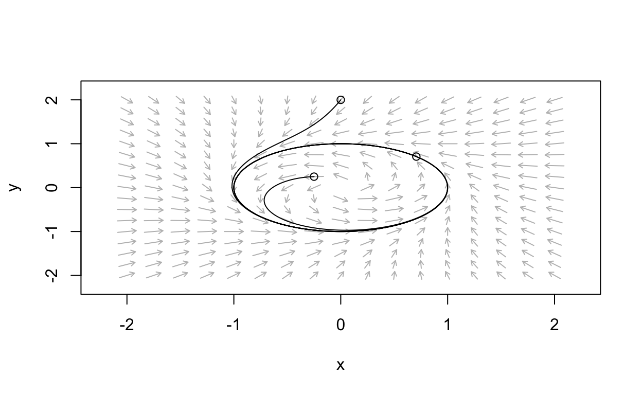
What happens if μ>0? Intuitively, we expect the persistence of a stable limit cycle, at least for small values of μ. This is because if we gradually make a small change to a continuous system there should not be a dramatic change in the results. Let’s compute an example with μ=0.5.

Show code

new_nonlinear_flowfield  <- flowField(pb_example ,
                                       xlim       = c(-2, 2),
                                       ylim       = c(-2, 2),
                                       parameters = c(mu=0.5),
                                       points     = 17,
                                       add = FALSE)
state <- matrix(c(-0.25,0.25,1.0/sqrt(2.0),1.0/sqrt(2.0),0.0,2.0),3,2,byrow = TRUE)

new_nonlinear_trajs <- trajectory(pb_example,
                                        y0         = state,
                                        tlim       = c(0, 10),
                                        parameters = c(mu=0.5),add=TRUE)

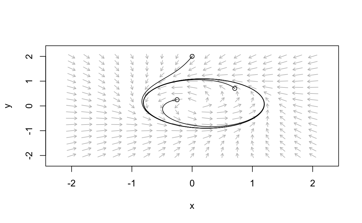
The stable limit cycle persist. Although it is difficult to see, the shape of the limit cycle has changed slightly when the μ=0.5 case is compared with that of the μ=0 case. Let’s return to the equations

drdt=r(1−r2)+μrcos(θ)dθdt=1

When μ≠0 the equation for the rate of change in the radial direction no longer decouples from the equation for the rate of change in the angular direction due to the presence of the rcos(θ) part. Thus, we can not as easily see that the system possesses a stable limit cycle. As we will show, the Poincarè-Bendixson theorem is a relatively simple tool that can be used to derive the existence of a stable limit cycle for a system like the one above even when μ>0. In the following section, we will state the theorem as in (Strogatz 2015) and then apply it to our example system.

The Poincarè-Bendixson Theorem

Consider a nonlinear autonomous two-dimensional system of the form

dxdt=f(x,y)dydt=g(x,y)

and suppose that R is a closed, bounded subset of the plan such that R is contained in a domain for the system upon which it is differentiable. Further, suppose that R does not contain any equilibrium points of the system.Then, if there exists a trajectory C that is confined in R so that if it starts in R it stays in R as t→∞, then either C is a closed orbit, or it spirals toward a closed orbit as t→∞. This setup and conclusion is the result known as the Poincarè-Bendixson theorem.

A region R satisfying the properties just described is sometimes known as a trapping region. Often, the key to an effective application of the Poincarè-Bendixson theorem is in the construction of an appropriate trapping region. This technique is illustrated by the following example.

Example

Consider again the system in polar coordinates,

drdt=r(1−r2)+μrcos(θ)dθdt=1

Note that the only equilibrium for this system is the point r=0.

Now, since −1≤cos(θ)≤1 and r≥0, then for any μ≥0 we have

r(1−r2)−μr≤r(1−r2)+μrcos(θ)≤r(1−r2)+μr

We are going to use this observation in order to try to find two concentric circles such that on the outer radius rout we have that rout(1−r2out)+μroutcos(θ)<0, and on the inner radius rin we have that 0<rin(1−r2in)+μrincos(θ). If this is the case, then we can conclude that trajectories on the inner radius are directed away from the origin, and trajectories on the outer radius are directed toward the origin. This makes R={r|rin≤r≤rout} a suitable trapping region because no trajectory that starts within R can exit it.

To complete the analysis, note that if r(1−r2)+μr<0, then r(1−r2)+μrcos(θ) is certainly negative. On the other hand, if 0<r(1−r2)−μr, then r(1−r2)+μrcos(θ) is certainly positive. We have that

r(1−r2)+μr<0 whenever √1+μ<r

and

0<r(1−r2)−μr<0 whenever r<√1−μ

Thus, we can take something like

rin=0.999√1−μ

provided that 0<μ<1, and

rout=1.001√1+μ.

We conclude that whenever 0<μ<1 we have a trapping region given by rin≤r≤rout. All of the other qualifications necessary for the Poincarè-Bendixson theorem to apply are met for trivial reasons thus there must be a closed orbit in the form of a stable limit cycle for the system

drdt=r(1−r2)+μrcos(θ)dθdt=1

Additional examples using the Poincarè-Bendixson theorem and some biomathematical applications of the technique will be provided during in-class lecture.

Further Reading

For further details on the topics covered in this section of notes, see Chapter 7 from (Strogatz 2015).