Goals
After reading this section of notes, you should
- have a greater appreciation for the application of the phase-plane methods covered in notes 11 and notes 12 in biomathematics.
Background
Mathematical models for biological systems often involve interacting variables. Such models take the form of a coupled system of nonlinear (typically autonomous) differential equations. When the system is of size two, phase-plane methods can be exploited to obtain information about the biological system being modeled. Even for higher-dimensional systems, phase-plane methods may still be useful and make it easier for us to understand what goes on in fairly complicated mathematical models.
In this section of notes, we will apply our phase-plane methods to analyze three models. We begin with a simple model for the populations of interacting species, then consider a variation on the general competition model we briefly introduced in our discussion of compartment models. Finally, we analyze the chemostat model for the nutrient limited growth of a bacterial cell population.
A Simple Two-Species Population Model
Consider the system
\[ \begin{align} \frac{dx}{dt} &= (3-x)x - 2xy = x(3-x-2y)\\ \frac{dy}{dt} &= (2-y)y - xy = y(2-x-y) \end{align} \] We can view this as a population model for the interacting species with populations \(x\) and \(y\). Basically what this model says is that both species follow logistic growth in the absence of the other species, but then there is competition that results in a death rate that is proportional to the population of the other species. This example is taken from section 6.4 of (Strogatz 2015).
Equilibrium points
Equilibrium points for the system satisfy
\[ \begin{align} 0 &= x(3-x-2y)\\ 0 &= y(2-x-y) \end{align} \] from which we can easily see that
\((x^{\ast},y^{\ast})=(0,0)\)
\((x^{\ast},y^{\ast})=(0,2)\)
\((x^{\ast},y^{\ast})=(3,0)\)
\((x^{\ast},y^{\ast})=(1,1)\)
are equilibrium points. In the context of the population model, the equilibrium point \((1,1)\) is called the coexistence steady-state because in all of the other three equilibrium points at least one species dies out.
Let’s confirm our equilibrium values by plotting the nullclines for the system.
Show code
simple_pop <- function(t,state,parameters){
  with(as.list(c(state,parameters)),{

    dx <- state[1]*(3-state[1]-2*state[2])
    dy <- state[2]*(2-state[1]-state[2])

    list(c(dx,dy))
  })
}

nonlinear_flowfield  <- flowField(simple_pop ,
                                       xlim       = c(-0.25, 4),
                                       ylim       = c(-0.25, 4),
                                       parameters = NULL,
                                       points     = 17,
                                       add = FALSE)
nonlinear_nullclines  <- nullclines(simple_pop,
                                       xlim       = c(-0.25, 4),
                                       ylim       = c(-0.25, 4),
                                       points=100,add.legend=FALSE)
eq1 <- findEquilibrium(simple_pop, y0 = c(0,0),
  plot.it = TRUE,summary=FALSE)
eq2 <- findEquilibrium(simple_pop, y0 = c(0,2),
  plot.it = TRUE,summary=FALSE)
eq3 <- findEquilibrium(simple_pop, y0 = c(3,0),
  plot.it = TRUE,summary=FALSE)
eq4 <- findEquilibrium(simple_pop, y0 = c(1,1),
  plot.it = TRUE,summary=FALSE)
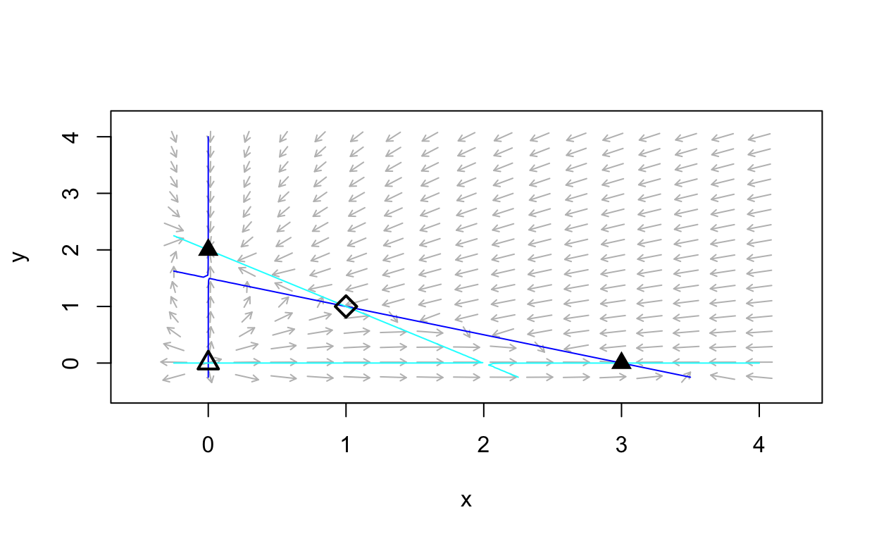
We do in fact see the four equilibrium values that we calculated. Further, we can see the nullclines and since they do not intersect in more than four points, we conclude that we have found all of the equilibrium values.
Linear stability analysis
In general we have that
\[ J_{(x,y)} = \left(\begin{array}{cc} 3-2x-2y & -2x \\ -y & 2-x-2y \end{array}\right) \]
and thus
\(J_{(0,0)} = \left(\begin{array}{cc} 3 & 0 \\ 0 & 2 \end{array}\right)\), which has \(\tau=5\), \(\delta=6\), and \(\delta < \frac{1}{4}\tau^2\).
\(J_{(0,2)} = \left(\begin{array}{cc} -1 & 0 \\ -2 & -2 \end{array}\right)\), which has \(\tau=-3\), \(\delta=2\), and \(\delta < \frac{1}{4}\tau^2\).
\(J_{(3,0)} = \left(\begin{array}{cc} -3 & -6 \\ 0 & -1 \end{array}\right)\), which has \(\tau=-4\), \(\delta=3\), and \(\delta < \frac{1}{4}\tau^2\).
\(J_{(1,1)} = \left(\begin{array}{cc} -1 & -2 \\ -1 & -1 \end{array}\right)\), which has \(\tau=-2\) and \(\delta=-1\).
Thus, using the trace-determinant plane implies that the results of our linear stability analysis are:
\((0,0)\) is an unstable node,
\((0,2)\) is a stable node,
\((3,0)\) is a stable node, and
\((1,1)\) is a saddle.
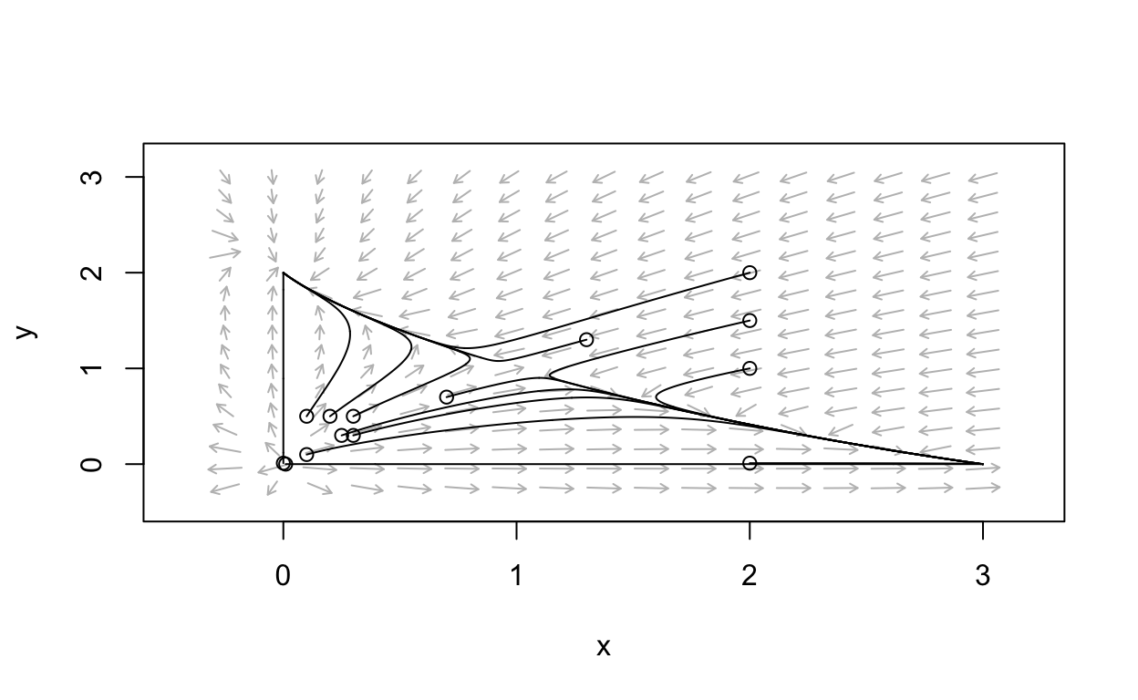
Phase portrait
We can easily obtain the phase portrait for the system
\[ \begin{align} \frac{dx}{dt} &= x(3-x-2y)\\ \frac{dy}{dt} &= y(2-x-y) \end{align} \]
using phaseR:
Conclusions
For the model system,
\[ \begin{align} \frac{dx}{dt} &= x(3-x-2y)\\ \frac{dy}{dt} &= y(2-x-y) \end{align} \] we conclude the following: Coexistence of the two species is theoretically possible. However, it is very delicate in the sense that the starting values for the two populations that will lead to co-existence is very limited. Most initial populations are such that one population out-competes the other. Which population wins out in competition depends solely on the relative starting size of the two species.
An obvious question is, are there competition models in which there is a robust co-existence equilibrium? Consideration of this question is taken up in the next section.
A More General Competition Model
This section follows section 2.5 from (Britton 2003). A mathematical model for intraspecific competition is
\[ \begin{align} \frac{du}{dt} &= r_{1}u\left(1 - \frac{u+\alpha v}{K_{1}} \right) \\ \frac{dv}{dt} &= r_{2}v\left(1 - \frac{v+\beta u}{K_{2}} \right) \end{align} \]
where \(u\) and \(v\) are the populations of two species in competition. The parameters \(\alpha\) and \(\beta\) are so-called competition coefficients.
Non-dimensionalization
We begin our analysis by non-dimensionalizing the system using the scalings \(x=\frac{u}{K_{1}}\), \(y=\frac{v}{K_{2}}\), and \(\tau=r_{1}t\).
Then,
\[ \begin{align} \frac{dx}{d\tau} &= \frac{dt}{d\tau}\frac{dx}{dt} \\ &= \frac{1}{r_{1}}\frac{d}{dt}\frac{u}{K_{1}} \\ &= \frac{1}{r_{1}K_{1}}\left( r_{1}u\left(1 - \frac{u+\alpha v}{K_{1}} \right) \right) \\ &= x\left(1 - \frac{K_{1}x + \alpha K_{2} y}{K_{1}} \right) \\ &= x\left(1 - x - \alpha\frac{K_{2}}{K_{1}}y \right) \end{align} \]
and
\[ \begin{align} \frac{dy}{d\tau} &= \frac{dt}{d\tau}\frac{dy}{dt} \\ &= \frac{1}{r_{1}}\frac{d}{dt}\frac{v}{K_{2}} \\ &= \frac{1}{r_{1}K_{2}}\left( r_{2}v\left(1 - \frac{v+\beta u}{K_{2}} \right) \right) \\ &= \frac{r_{1}}{r_{2}}y\left(1 - \frac{K_{2}y+\beta K_{1} x}{K_{2}} \right) \\ &= \frac{r_{1}}{r_{2}}y\left(1 - y - \beta \frac{K_{1}}{K_{2}}x \right) \end{align} \] From the two previous derivations we conclude
\[ \begin{align} \frac{dx}{d\tau} &= x(1 - x - ay) \\ \frac{dy}{d\tau} &= cy(1 - bx - y) \end{align} \]
where \(a=\alpha\frac{K_{2}}{K_{1}}\), \(b=\beta\frac{K_{1}}{K_{2}}\), and \(c=\frac{r_{1}}{r_{2}}\).
Equilibrium points
Our analysis proceeds by determining the equilibrium points for
\[ \begin{align} \frac{dx}{d\tau} &= x(1 - x - ay) \\ \frac{dy}{d\tau} &= cy(1 - bx - y) \end{align} \] obtained by solving
\[ \begin{align} 0 &= x(1 - x - ay) \\ 0 &= cy(1 - bx - y) \end{align} \] leading to equilibrium points \((0,0)\), \((0,1)\), \((1,0)\), and \(\left(\frac{1-a}{1-ab},\frac{1-b}{1-ab}\right)\). The coexistence steady-state is \(\left(\frac{1-a}{1-ab},\frac{1-b}{1-ab}\right)\) and it is the one we are most interested in. Note that it is only biologically realistic if either \(a<1\) and \(b<1\), or \(a>1\) and \(b>1\).
Linear stability analysis
We want to determine if there are any conditions in which the coexistence steady-state \(\left(\frac{1-a}{1-ab},\frac{1-b}{1-ab}\right)\) is stable. Generically, we have
\[ J_{(x,y)} = \left(\begin{array}{cc} 1-2x-ay & -ax \\ -bcy & c(1-bx-2y) \end{array}\right) \] and thus
\[ J_{(x^{\ast},y^{\ast})} = J_{\left(\frac{1-a}{1-ab},\frac{1-b}{1-ab}\right)} = \left(\begin{array}{cc} -\frac{1-a}{1-ab} & -a\frac{1-a}{1-ab} \\ -bc\frac{1-b}{1-ab} & -c\frac{1-b}{1-ab} \end{array}\right) \] Now, the coexistence steady-state will be stable if the trace of the previous matrix is negative and its determinant is positive. It is obvious that is either \(a<1\) and \(b<1\), or \(a>1\) and \(b>1\), then the trace will be negative since
\[\text{tr}(J_{(x^{\ast},y^{\ast})}) = -\frac{1-a}{1-ab}-c\frac{1-b}{1-ab} < 0\] The determinant is
\[ \begin{align} \text{det}(J_{(x^{\ast},y^{\ast})}) &= \frac{c(1-a)(1-b)}{(1-ab)^2} - \frac{abc(1-a)(1-b)}{(1-ab)^2} \\ &= \frac{c(1-a)(1-b)}{(1-ab)^2}(1-ab) \end{align} \]
This will be positive if \(a<1\) and \(b<1\). Thus,
The coexistence steady-state exists and is stable if \(a<1\) and \(b<1\).
What does this mean in the context of the original model
\[ \begin{align} \frac{du}{dt} &= r_{1}u\left(1 - \frac{u+\alpha v}{K_{1}} \right) \\ \frac{dv}{dt} &= r_{2}v\left(1 - \frac{v+\beta u}{K_{2}} \right) \end{align} \]
Recall that \(a=\alpha\frac{K_{2}}{K_{1}}\) and \(b=\beta\frac{K_{1}}{K_{2}}\). Notice that if \(a<1\) and \(b<1\), then
\(1 > ab = \alpha\frac{K_{2}}{K_{1}} \beta\frac{K_{1}}{K_{2}} = \alpha \beta\).
Thus, when we have a stable coexistence steady-state we have \(\alpha \beta < 1\).
Example phase portrait
Here is an example phase portrait for a system of the form
\[ \begin{align} \frac{dx}{d\tau} &= x(1 - x - ay) \\ \frac{dy}{d\tau} &= cy(1 - bx - y) \end{align} \]
with \(a<1\) and \(b<1\).
Show code
nonlinear_example <- function(t,state,parameters){
  with(as.list(c(state,parameters)),{

    dx <- state[1]*(1-state[1]-a*state[2])
    dy <- c*state[2]*(1-b*state[1]-state[2])

    list(c(dx,dy))
  })
}

nonlinear_flowfield  <- flowField(nonlinear_example,
                                       xlim       = c(-0.25, 1.5),
                                       ylim       = c(-0.25, 1.5),
                                       parameters = c(a=0.25,b=0.75,c=1.0),
                                       points     = 17,
                                       add = FALSE)
state <- matrix(c(0.1,0.1,0.5,0.1,0.1,0.5,0.5,0.5,
                  0.5,0.75,0.75,0.5,1.0,1.0,0.75,1.0,1.5,0.5),9,2,byrow = TRUE)
nonlinear_trajs <- trajectory(nonlinear_example,
                                        y0         = state,
                                        tlim       = c(0, 10),
                                        parameters = c(a=0.25,b=0.75,c=1.0),add=TRUE)
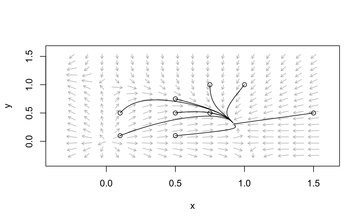
It is clear that there is a stable equilibrium point with both components being positive values.
Conclusions
We have derived a condition for the existence of a stable coexistence steady-state. There is a further consequence of this analysis. Generally, two species with populations that obey
\[ \begin{align} \frac{du}{dt} &= r_{1}u\left(1 - \frac{u+\alpha v}{K_{1}} \right) \\ \frac{dv}{dt} &= r_{2}v\left(1 - \frac{v+\beta u}{K_{2}} \right) \end{align} \]
occupy the same ecological niche if \(\alpha \beta = 1\). If they coexist, then \(\alpha \beta < 1\). Therefore, competitors can not occupy the same ecological niche. This is a proof of the so-called principle of competitive exclusion.
Chemostat Model
For our final example, consider the chemostat model with non-dimensional form
\[ \begin{align} \frac{dx}{d\tau} &= a_{1} \frac{y}{1 + y} x - x \\ \frac{dy}{d\tau} &= - \frac{y}{1 + y} x - y + a_{2} \end{align} \]
Here, \(a_{1}\) and \(a_{2}\) are positive constants. The following analysis roughly follows that found in section 4.10 of (Edelstein-Keshet 2005).
Equilibrium points
Equilibrium points are determined by solutions to the system
\[ \begin{align} 0 &= a_{1} \frac{y}{1 + y} x - x = x\left(a_{1}\frac{y}{1+y} - 1 \right) \\ 0 &= - \frac{y}{1 + y} x - y + a_{2} \end{align} \] From the first equation, we see that we must have either \(x=0\) or \(a_{1}\frac{y}{1+y} - 1=0\). In case \(x=0\), equation the second equation implies that \(y=a_{2}\). Thus, one equilibrium value is
- \((x^{\ast},y^{\ast})=(0,a_{2})\).
On the other have, if \(a_{1}\frac{y}{1+y} - 1=0\), then \(y = \frac{1}{a_{1} - 1}\). Solving the second equation for \(x\) gives
\[ \begin{align} x &= \frac{1+y}{y}(a_{2}-y) \\ &= \frac{1+\frac{1}{a_{1} - 1}}{\frac{1}{a_{1} - 1}}\left(a_{2} - \frac{1}{a_{1} - 1} \right) \\ &= (a_{1} - 1 + 1)\left(a_{2} - \frac{1}{a_{1} - 1} \right) \\ &= a_{1}\left( \frac{a_{2}(a_{1}-1) - 1}{a_{1} - 1} \right) \end{align} \] Thus, we have a second equilibrium value
- \((x^{\ast},y^{\ast})=\left(a_{1}\left( \frac{a_{2}(a_{1}-1) - 1}{a_{1} - 1}\right),\frac{1}{a_{1} - 1} \right)\)
In the context of the biological system, only non-negative equilibrium values are relevant. Therefore, we only consider the second equilibrium whenever
\(a_{1} > 1\), and
\(a_{2}(a_{1}-1) > 1\)
Linear stability analysis
Let’s consider the linearization of the chemostat model at the equilibrium points. First, note that
\[ J_{(x,y)} = \left(\begin{array}{cc}a_{1}\frac{y}{1+y}-1 & a_{1}x\frac{1}{(1+y)^2} \\ -\frac{y}{1+y} & -x\frac{1}{(1+y)^{2}} - 1 \end{array}\right) \] Now observe that if \(y=\frac{1}{a_{1}-1}\), then
\(\frac{y}{1+y} = \frac{1}{a_{1}}\)
and
\(\frac{1}{(1+y)^2}=\left(\frac{a_{1}-1}{a_{1}} \right)^2\)
Therefore,
\[ J_{\left(a_{1}\left( \frac{a_{2}(a_{1}-1) - 1}{a_{1} - 1}\right),\frac{1}{a_{1} - 1} \right)} = \left(\begin{array}{cc} 0 & (a_{1}-1)(a_{2}(a_{1} -1 ) - 1) \\ -\frac{1}{a_{1}} & -(a_{2}(a_{1}-1) - 1)\left(\frac{a_{1}-1}{a_{1}}\right) - 1 \end{array}\right) \]
Now, this matrix has
trace \(\tau = -(a_{2}(a_{1}-1) - 1)\left(\frac{a_{1}-1}{a_{1}}\right) - 1 < 0\), and
determinant \(\delta = \frac{(a_{1}-1)(a_{2}(a_{1} -1 ) - 1)}{a_{1}} > 0\)
from which we can conclude that \(\left(a_{1}\left( \frac{a_{2}(a_{1}-1) - 1}{a_{1} - 1}\right),\frac{1}{a_{1} - 1} \right)\) is a stable equilibrium (provided it exists as a positive equilibrium).
Finally, define \(A = \frac{(a_{1}-1)(a_{2}(a_{1} -1) - 1)}{a_{1}}\), then we can write \(\tau=-A-1\) and \(\delta = A\), then
\(\tau^2 - 4\delta = (A+1)^2-4A = A^{2} + 2A + 1 - 4A = A^2 - 2A + 1 = (A-1)^2 > 0\)
from which we conclude that \(\left(a_{1}\left( \frac{a_{2}(a_{1}-1) - 1}{a_{1} - 1}\right),\frac{1}{a_{1} - 1} \right)\) is a stable node.
Example phase portrait
Show code
chemostat_example <- function(t,state,parameters){
  with(as.list(c(state,parameters)),{

    dx <- state[1]*(a1*state[2]/(1+state[2]) - 1)
    dy <- -state[1]*state[2]/(1+state[2]) - state[2] + a2

    list(c(dx,dy))
  })
}

nonlinear_flowfield  <- flowField(chemostat_example ,
                                       xlim       = c(-0.25, 2.5),
                                       ylim       = c(-0.25, 2.5),
                                       parameters = c(a1=2.5,a2=1.5),
                                       points     = 17,
                                       add = FALSE)
state <- matrix(c(0.1,0.1,0.5,0.1,0.1,0.5,0.5,0.5,
                  0.5,0.75,0.75,0.5,1.0,1.0,0.75,
                  1.0,1.5,0.5,2.5,1.0,2.0,2.0,2.5,0.25,1.5,1.5),13,2,byrow = TRUE)
nonlinear_trajs <- trajectory(chemostat_example ,
                                        y0         = state,
                                        tlim       = c(0, 10),
                                        parameters = c(a1=2.5,a2=1.5),add=TRUE)
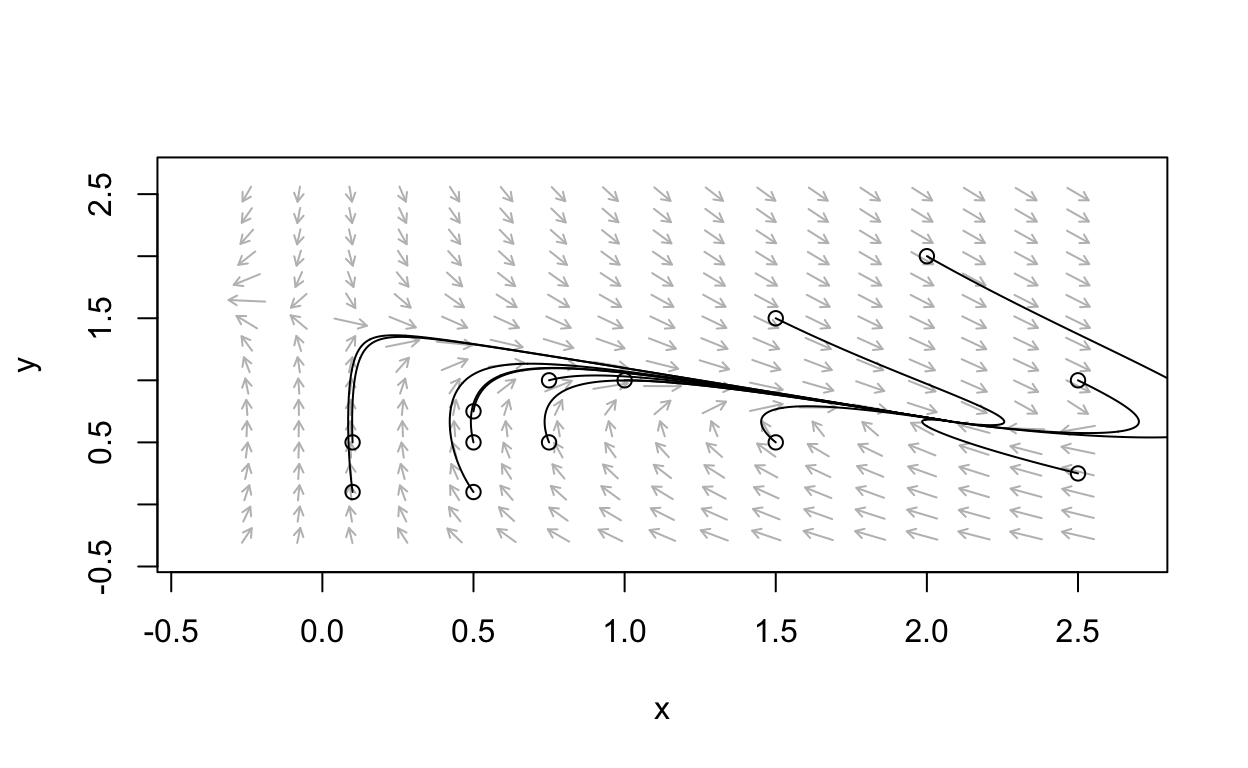
We see that there is in fact an equilibrium point that is a stable node.
Conclusions
We have shown that there are conditions that result in long-term positive values for both a bacteria cell population and nutrient concentration. These are \(a_{1} > 1\) and \(a_{2}(a_{1}-1) > 1\). Recall that in our non-dimensionalization we determined
\(a_{1} = \frac{K_{\text{max}}V}{F}\)
and
\(a_{2}=\frac{C_{0}}{k_{n}}\)
Thus, we must have
\(K_{\text{max}} < \frac{F}{V}\)
and
\(\frac{F}{V}\frac{k_{n}}{K_{\text{max}} - \frac{F}{V}} < C_{0}\)
in order to get a stable positive steady-state solution to the chemostat model.