Goals
After reading this section of notes, you should
be able to conduct a linear stability analysis for a nonlinear autonomous system,
know how to use
phaseRto obtain phase-portraits for two-dimensional nonlinear systems, andknow how to compute numerical solutions for initial value problems for nonlinear systems using
deSolve.
Background
Previously, we have reviewed mathematical techniques for the analysis of one-dimensional autonomous systems and linear systems. In this section, we consider the analogous techniques for nonlinear autonomous systems of the form
\[ \frac{d}{dt}{\bf x} = {\bf F}({\bf x}) \]
where \({\bf x} \in \mathbb{R}^n\) and \({\bf F}:\mathbb{R}^n \rightarrow \mathbb{R}^n\). Such a system is sometimes called a nonlinear vector field.
We have already encountered some nonlinear autonomous systems as mathematical models. For example, the predator-prey model, SIR model, and chemostat model are all nonlinear autonomous systems.
Equilibria for Nonlinear Systems
If \(\frac{d}{dt}{\bf x} = {\bf F}({\bf x})\) is a nonlinear autonomous system, then we say that a vector \({\bf x}^{\ast}\) is an equilibrium if it satisfies \({\bf F}({\bf x}^{\ast}) = {\bf 0}\). A typical problem is to determine the stability properties of equilibria for nonlinear systems. In general this can be a difficult problem. However, in some cases when can use linearization to say something about the stability of equilibria. We begin by reviewing this technique in the two-dimensional case.
Two-Dimensional Case
We can write a two-dimensional nonlinear autonomous system as
\[ \begin{align*} \frac{dx}{dt} &= f(x,y) \\ \frac{dy}{dt} &= g(x,y) \end{align*} \]
Then an equilibrium is a point \((x^{\ast},y^{\ast})\) satisfying the simultaneous system
\[ \begin{align*} f(x^{\ast},y^{\ast}) &= 0 \\ g(x^{\ast},y^{\ast}) &= 0 \end{align*} \]
For example, the system
\[ \begin{align*} \frac{dx}{dt} &= 2x - 3xy \\ \frac{dy}{dt} &= xy - 4y \end{align*} \]
has two equilibria, \((0,0)\) and \((4,\frac{3}{2})\).
If \((x^{\ast},y^{\ast})\) is an equilibrium point for a two-dimensional nonlinear autonomous system, then we call the matrix
\[ J_{(x^{\ast},y^{\ast})} = \left(\begin{array}{cc} f_{x}(x^{\ast},y^{\ast}) & f_{y}(x^{\ast},y^{\ast}) \\ g_{x}(x^{\ast},y^{\ast}) & g_{y}(x^{\ast},y^{\ast}) \end{array} \right) \]
the linearization of the system at the equilibrium \((x^{\ast},y^{\ast})\). It turns out that in some cases, the linearization can be used to determine the stability of the equilibrium \((x^{\ast},y^{\ast})\). Specifically, if the eigenvalues of \(J_{(x^{\ast},y^{\ast})}\) have nonzero real part, then near the equilibrium, the system behaves exactly as the corresponding linear system \(\frac{d}{dt}{\bf x}= J_{(x^{\ast},y^{\ast})}{\bf x}\) behaves. This is a result known as the Hartman-Grobman theorem.
Consider again the example system
\[ \begin{align*} \frac{dx}{dt} &= 2x - 3xy \\ \frac{dy}{dt} &= xy - 4y \end{align*} \]
which possesses equilibria \((0,0)\) and \((4,\frac{3}{2})\). Then
\[ J(0,0) = \left(\begin{array}{cc} 2 & 0 \\ 0 & -4 \end{array} \right), \ \ \ J(4,\frac{3}{2}) = \left(\begin{array}{cc} 0 & -12 \\ \frac{3}{2} & 0 \end{array} \right) \] For the linearization \(J(0,0)\), the eigenvalues are \(2\) and \(-4\). Thus, we conclude that there is a saddle at \((0,0)\). On the other hand, the eigenvalues of \(J(4,\frac{3}{2})\) are \(\pm i 3\sqrt{2}\) which have zero real part and thus are pure imaginary. The Hartman-Grobman theorem does no apply and does not allow us to conclude the dynamics near \((4,\frac{3}{2})\).
Phase-Portaits
It is possible to study two-dimensional autonomous systems geometrically analogous to what we did with one-dimesional autonomous systems. But in this case, we draw a phase-plane instead of a phase-line. To understand this, first note that a solution to the system
\[ \begin{align*} \frac{dx}{dt} &= f(x,y) \\ \frac{dy}{dt} &= g(x,y) \end{align*} \] with initial condition \((x_{0},y_{0})\) will be a parametric curve in the plane passing through the point \((x_{0},y_{0})\). We refer to such as curve as a trajectory of the system, The right hand side of the system determines a vector field and these vectors are tangent to trajectories. Thus, if we plot the vector field, then we can see all of the trajectories by following vectors tangentially.
For example, the following plot shows the vector field for
\[ \begin{align*} \frac{dx}{dt} &= 2x - 3xy \\ \frac{dy}{dt} &= xy - 4y \end{align*} \]Show code
nonlinear_example <- function(t,state,parameters){
  with(as.list(c(state,parameters)),{

    dx <- 2*state[1] - 3*state[1]*state[2]
    dy <- state[1]*state[2] - 4*state[2]

    list(c(dx,dy))
  })
}

nonlinear_flowfield  <- flowField(nonlinear_example,
                                       xlim       = c(-0.5, 4.5),
                                       ylim       = c(-0.5, 3),
                                       parameters = NULL,
                                       points     = 17,
                                       add = FALSE)
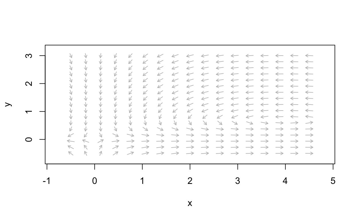
It is easy to see that there is a saddle point at \((0,0)\). Furthermore, from the vector field it appears that there are rotations around \((4,\frac{3}{2})\) which suggests either a sprial or perhaps a nonlinear center. We will explore this further soon. First, reacll that if \[ \begin{align*} \frac{dx}{dt} &= f(x,y) \\ \frac{dy}{dt} &= g(x,y) \end{align*} \]
is a nonlinear system, the setting each component of the vector field to zero determines curves. Thus there are \(f(x,y)=0\) curves and \(g(x,y)=0\) curves. Such curves are called nullclines. This is due to the fact that along a \(f(x,y)=0\) curve, we have that \(\frac{dx}{dt}=0\) and hence there is no change in the \(x\) direction. On the other hand, along a \(g(x,y)=0\) curve, we have that \(\frac{dy}{dt}=0\) and hence there is no change in the \(y\) direction. Note that equilibria points are exactly intersectoin points of distinct nullclines. The following plot shows the nullclines for the example system
\[ \begin{align*} \frac{dx}{dt} &= 2x - 3xy \\ \frac{dy}{dt} &= xy - 4y \end{align*} \]
Show code
nonlinear_flowfield  <- flowField(nonlinear_example,
                                       xlim       = c(-0.5, 4.5),
                                       ylim       = c(-0.5, 3),
                                       parameters = NULL,
                                       points     = 17,
                                       add = FALSE)
nonlinear_nullclines  <- nullclines(nonlinear_example,
                                       xlim       = c(-0.5, 4.5),
                                       ylim       = c(-0.5, 3),
                                       points=100,add.legend=FALSE)
eq1 <- findEquilibrium(nonlinear_example, y0 = c(0,0),
  plot.it = TRUE,summary=FALSE)
eq2 <- findEquilibrium(nonlinear_example, y0 = c(4,3/2),
  plot.it = TRUE,summary=FALSE)
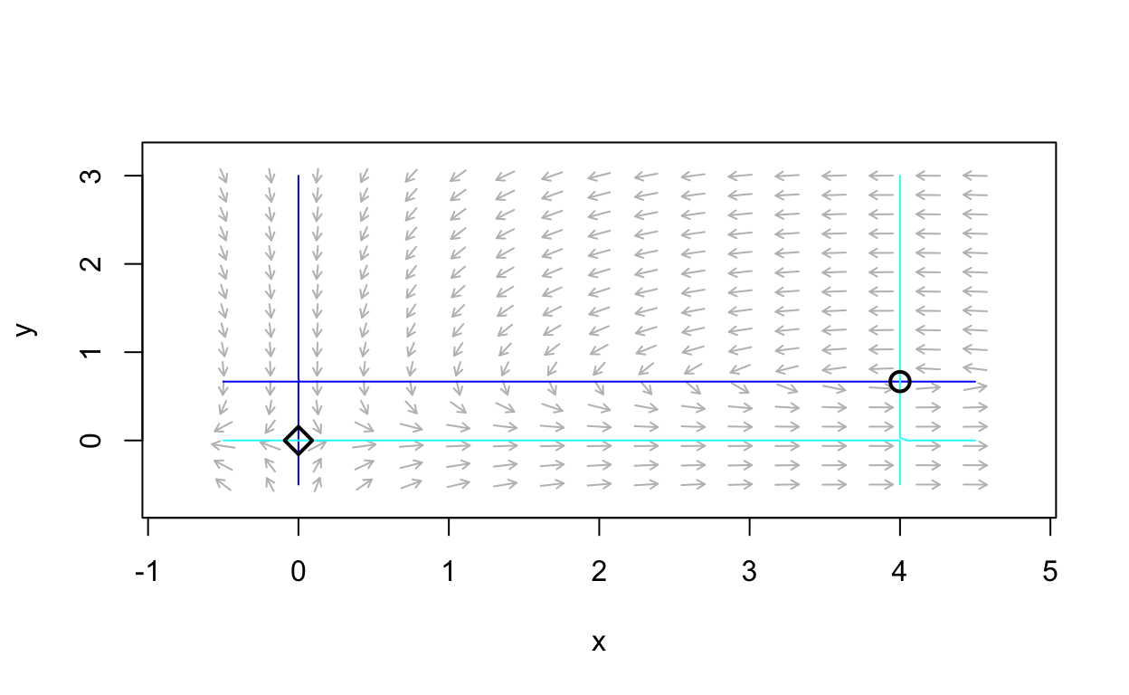
We can see the equilibrium points at the intersection of distinct nullclines. Let’s plot several trajectories to obtain a phase-portrait.
Show code
nonlinear_flowfield  <- flowField(nonlinear_example,
                                       xlim       = c(-0.5, 4.5),
                                       ylim       = c(-0.5, 3),
                                       parameters = NULL,
                                       points     = 17,
                                       add = FALSE)
nonlinear_nullclines  <- nullclines(nonlinear_example,
                                       xlim       = c(-0.5, 4.5),
                                       ylim       = c(-0.5, 3),
                                       points=100,add.legend=FALSE)
eq1 <- findEquilibrium(nonlinear_example, y0 = c(0,0),
  plot.it = TRUE,summary=FALSE)
eq2 <- findEquilibrium(nonlinear_example, y0 = c(4,3/2),
  plot.it = TRUE,summary=FALSE)
state <- matrix(c(0.2,0.2,0.5,0.5,0,3,0,-1,0.01,0,-0.01,0,4,1.25),7,2,byrow = TRUE)
nonlinear_trajs <- trajectory(nonlinear_example,
                                        y0         = state,
                                        tlim       = c(0, 10),
                                        parameters = NULL,add=TRUE)
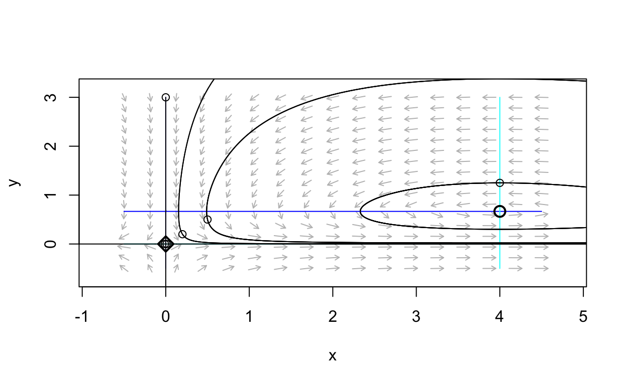
Notice that this system has trajectories that are closed curves in the plane. Thus, this system possesses periodic solutions. To confirm this, let’s plot the time-series for one of the trajectories that appears to correspond to a periodic solution. Namely, let’s plot the solution corresponding to initical condition \((4,1.25)\).
Show code
num_sol <- numericalSolution(nonlinear_example,y0=c(4,1.25),tlim=c(0,10))
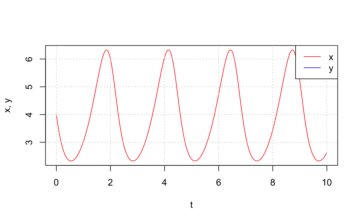
We will return to the topic of periodic solutions to nonlinear systems later. For now, note that linearization cannot typically be used to detect the existence of periodic solutions.
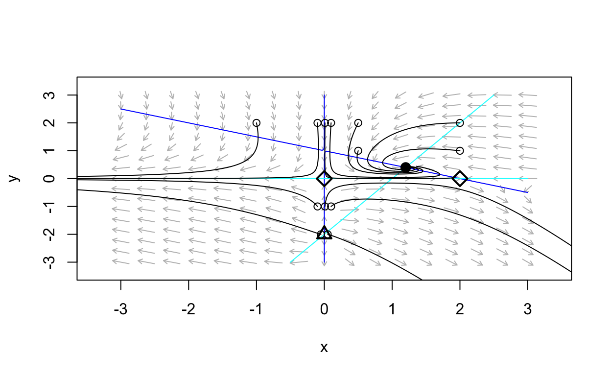
A Gallery of Two-Dimensional Systems
What follows is a sequence of examples of using phaseR
to produce a phase portrait for a two-dimensional nonlinear autonomous
system. As an exercise, you should attempt to determine the equilibria
and their stability properties for each system.
Show code
gallery_example_1 <- function(t,state,parameters){
  with(as.list(c(state,parameters)),{

    dx <- state[1]*(1 - 0.5*state[1] - state[2])
    dy <- state[2]*(state[1] - 1 - 0.5*state[2])

    list(c(dx,dy))
  })
}

nonlinear_flowfield  <- flowField(gallery_example_1,
                                       xlim       = c(-3, 3),
                                       ylim       = c(-3, 3),
                                       parameters = NULL,
                                       points     = 17,
                                       add = FALSE)
nonlinear_nullclines  <- nullclines(gallery_example_1,
                                       xlim       = c(-3, 3),
                                       ylim       = c(-3, 3),
                                       points=100,add.legend=FALSE)
eq1 <- findEquilibrium(gallery_example_1, y0 = c(0,0),
  plot.it = TRUE,summary=FALSE)
eq2 <- findEquilibrium(gallery_example_1, y0 = c(2,0),
  plot.it = TRUE,summary=FALSE)
eq3 <- findEquilibrium(gallery_example_1, y0 = c(0,-2),
  plot.it = TRUE,summary=FALSE)
eq4 <- findEquilibrium(gallery_example_1, y0 = c(6/5,2/5),
  plot.it = TRUE,summary=FALSE)
state <- matrix(c(-0.1,-1,-0.1,2,
                  0.01,-1,0.01,2,
                  0.1,-1,0.1,2,-0.05,-2,
                  0.5,1,0.05,-2,0.5,2,
                  2,1,2,2,-1,2),13,2,byrow = TRUE)
nonlinear_trajs <- trajectory(gallery_example_1,
                                        y0         = state,
                                        tlim       = c(0, 10),
                                        parameters = NULL,add=TRUE)
Show code
gallery_example_2 <- function(t,state,parameters){
  with(as.list(c(state,parameters)),{

    dx <- state[2]
    dy <- state[1]*(1 - state[1]^2) + state[2]

    list(c(dx,dy))
  })
}

nonlinear_flowfield  <- flowField(gallery_example_2,
                                       xlim       = c(-3, 3),
                                       ylim       = c(-3, 3),
                                       parameters = NULL,
                                       points     = 17,
                                       add = FALSE)
nonlinear_nullclines  <- nullclines(gallery_example_2,
                                       xlim       = c(-3, 3),
                                       ylim       = c(-3, 3),
                                       points=100,add.legend=FALSE)
eq1 <- findEquilibrium(gallery_example_2, y0 = c(0,0),
  plot.it = TRUE,summary=FALSE)
eq2 <- findEquilibrium(gallery_example_2, y0 = c(1,0),
  plot.it = TRUE,summary=FALSE)
eq3 <- findEquilibrium(gallery_example_2, y0 = c(-1,0),
  plot.it = TRUE,summary=FALSE)
state <- matrix(c(0.01,0.01,0.01,-0.01,-0.01,0.01,-0.01,-0.01,
                  -0.5,0.0,0.5,0.0,
                  -1,-0.1,-1,0.1,1,-0.1,1,0.1),10,2,byrow = TRUE)
nonlinear_trajs <- trajectory(gallery_example_2,
                                        y0         = state,
                                        tlim       = c(0, 10),
                                        parameters = NULL,add=TRUE)

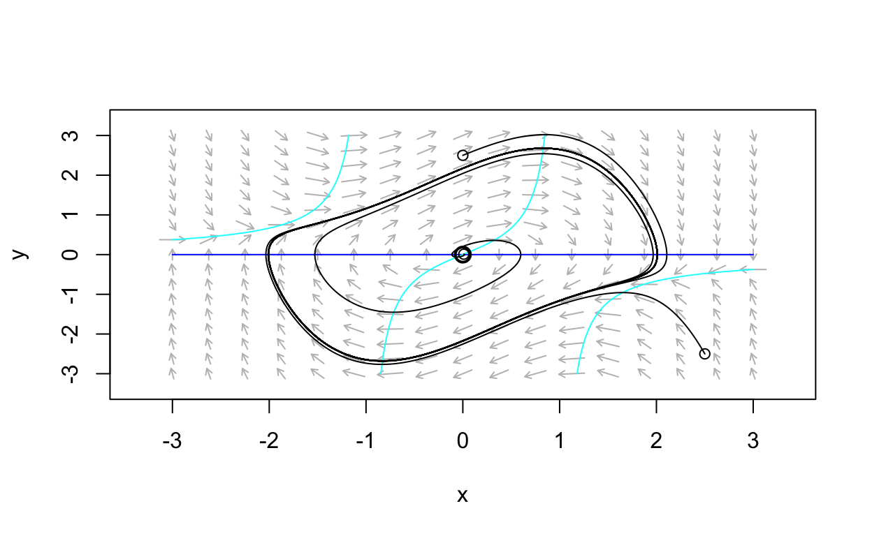
Show code
gallery_example_3 <- function(t,state,parameters){
  with(as.list(c(state,parameters)),{

    dx <- state[2]
    dy <- -state[1] + (1 - state[1]^2) * state[2]

    list(c(dx,dy))
  })
}

nonlinear_flowfield  <- flowField(gallery_example_3,
                                       xlim       = c(-3, 3),
                                       ylim       = c(-3, 3),
                                       parameters = NULL,
                                       points     = 17,
                                       add = FALSE)
nonlinear_nullclines  <- nullclines(gallery_example_3,
                                       xlim       = c(-3, 3),
                                       ylim       = c(-3, 3),
                                       points=100,add.legend=FALSE)
eq1 <- findEquilibrium(gallery_example_3, y0 = c(0,0),
  plot.it = TRUE,summary=FALSE)
state <- matrix(c(0.01,0.01,0,2.5,2.5,-2.5),3,2,byrow = TRUE)
nonlinear_trajs <- trajectory(gallery_example_3,
                                        y0         = state,
                                        tlim       = c(0, 50),
                                        parameters = NULL,add=TRUE)
Higher Dimensional Systems
As the dimension of a nonlinear system increases so does the
difficulty in analyzing the equilibria and their stability properties.
Once the dimension is three or greater, geometric analysis ranges from
very difficult to impossible. Thus, in Topics in Biomathematics
we will resign ourselves to handling larger nonlinear systems with
numerical computing using the deSolve package. We
illustrate this with an example.
Hodgkin-Huxley Model
Neuronal dynamics is concerned with the dynamical behavior of components of the nervous system and forms the basis for computational neuroscience. The starting point for this field of research is the Hodgkin-Huxley model for the neuron action potential. We will discuss this model in detail later. For now, we write down the equations mostly to note that the model is made up of a system of four nonlinear differential equations:
\[
\begin{align*}
C \frac{d}{dt}v &= g_{\text{na}} m^3 h (v_{\text{na}} - v) +
g_{\text{k}} n^4 (v_{\text{k}} - v) + g_{\text{l}} (v_{\text{l}} - v) +
i_{\text{ext}} \\
\frac{d}{dt}h &= \frac{h_{\text{inf}} - h}{\tau_{h}} \\
\frac{d}{dt}m &= \frac{m_{\text{inf}} - m}{\tau_{m}} \\
\frac{d}{dt}n &= \frac{n_{\text{inf}} - n}{\tau_{n}}
\end{align*}
\] The first equation is for the neuron action potential and the
other equations are called gating variables. The gating variables relate
to probabilities for various ions (electrically charged molecules) to
pass through the neuronal cell membrane. Here, we solve these equations
numerically just to illustrate how this can be done with
deSolve.
Show code
source("./R/gatingVariables.R")

# parameters
parameters <- list(C=1,gk=36,gna=120,gl=0.3,vk=-82,vna=45,vl=-59,iext=10)

# initial conditions
v0 <- -50
m0 <- alpha_m(v0)/(alpha_m(v0)+beta_m(v0));

yini <- c(v=v0, h=1, m=m0, n=0.4)


t_initial <- 0
t_final <- 75
times <- seq(from = t_initial, to = t_final, by = 0.08)


# define function to be in the format that `ode` uses
HH <- function (t, y, parameters) {
   with(as.list(c(y,parameters)),{
    # variables
    v <- y[1]
    h <- y[2]
    m <- y[3]
    n <- y[4]
    # functional forms
    h_inf <- alpha_h(v)/(alpha_h(v) + beta_h(v))
    m_inf <- alpha_m(v)/(alpha_m(v) + beta_m(v))
    n_inf <- alpha_n(v)/(alpha_n(v) + beta_n(v))

    tau_h <- 1/(alpha_h(v) + beta_h(v))
    tau_m <- 1/(alpha_m(v) + beta_m(v))
    tau_n <- 1/(alpha_n(v) + beta_n(v))

    dv <- (gna*m^3*h*(vna - v) + gk*n^4*(vk - v) + gl*(vl - v) + iext)/C
    dh <- (h_inf - h)/tau_h
    dm <- (m_inf - m)/tau_m
    dn <- (n_inf - n)/tau_n

    return(list(c(dv, dh, dm, dn)))
  })
}

out <- ode(y = yini, times = times, func = HH,
           parms = parameters,method = "ode45")
In order to run the code above, you need an R script
gatingVariables.R which is available here.
Let’s plot our results:
Show code
HHsol <- data.frame(t=out[,"time"],v=out[,"v"],h=out[,"h"],m=out[,"m"],n=out[,"n"])


p1 <- HHsol %>%
  ggplot(aes(x = t, y = v)) +
  geom_line(aes(x = t, y = v),lwd=1) +
  labs(x="time [ms]",y = "v [mV]") +
  theme_bw() + theme(text=element_text(size=20))

p2 <- HHsol %>%
  pivot_longer(-c(t,v),names_to="Variable", values_to="Value") %>%
  ggplot(aes(x = t, y = Value, color = Variable)) +
  geom_line(aes(x = t, y = Value),lwd=1) +
  labs(x="time [ms]",y = " ") +
  guides(color=guide_legend(title="Gating variable")) + theme(text=element_text(size=20))

(p1 / p2)
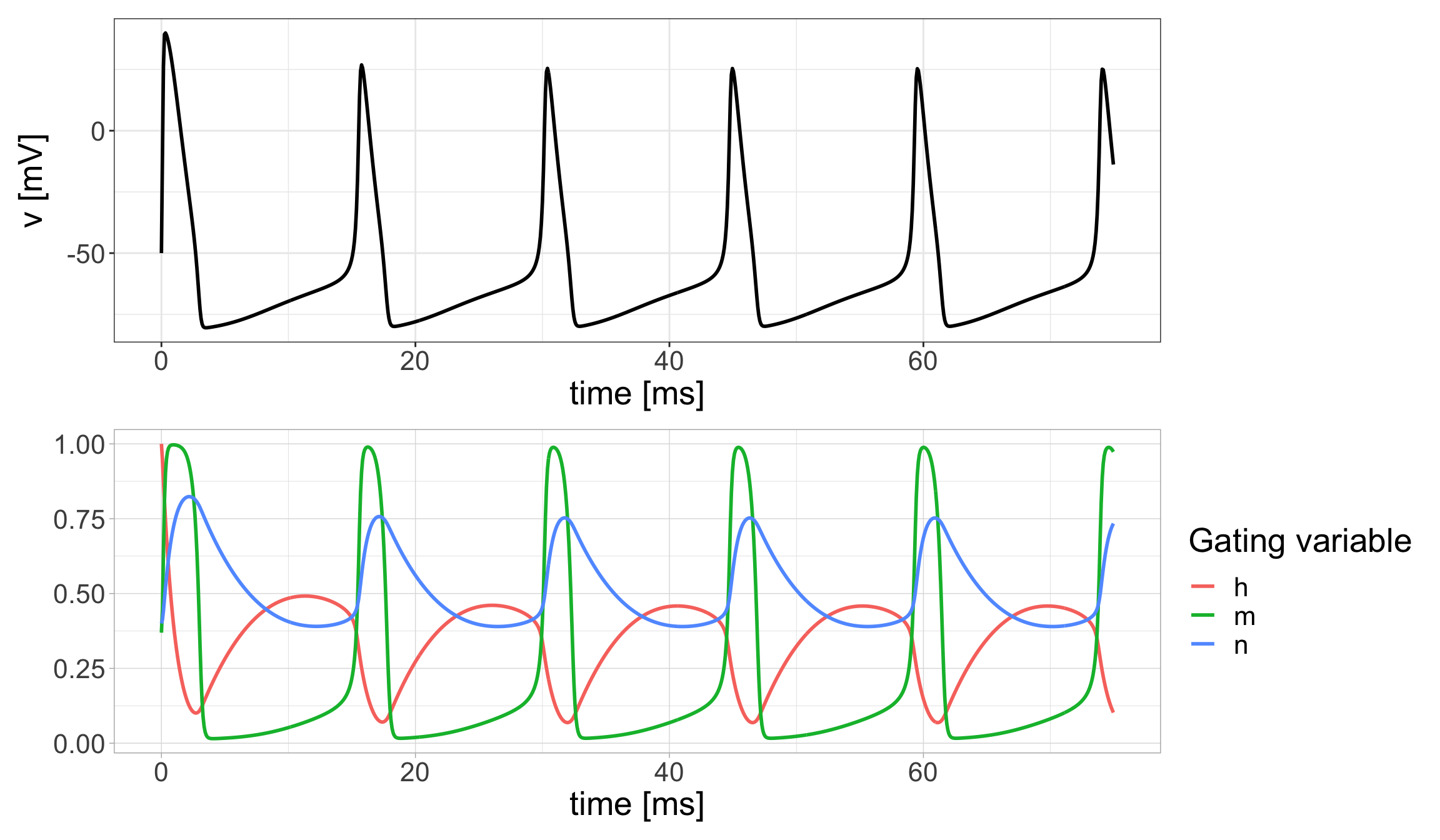
A distinct feature of the dynamics is the periodic nonlinear oscillations. We will have more to say about this later. From now on, anytime you encounter a model that is made up of large system of equations in Topics in Biomathematics, you should try to explore the model behavior by producing numerical solutions as we have done here with the Hodgkin-Huxley model.
Further Reading
For more information on the dynamics of nonlinear systems, we recommend the following sources (Allen 2007), (Barnes and Fulford 2015), (Britton 2003), (de Vries et al. 2006), (Edelstein-Keshet 2005), (Hirsch and Smale 1974), (Jones, Plank, and Sleeman 2010), (Strogatz 2015).
A good reference for the Hodgkin-Huxley model is (Börgers 2017).