Goals
After reading this section of notes, you should
know what a limit cycle is,
be able to rewrite a two-dimensional system in polar coordinates, and
understand the relationship between limit cycles and periodic solutions.
Background
In a previous note, we completely classified the possible phase portraits for a two-dimensional system of the form
\[ \left(\begin{array}{c} \frac{dx}{dt} \\ \frac{dy}{dt} \end{array} \right) = \left(\begin{array}{cc} a_{11} & a_{12} \\ a_{21} & a_{22} \end{array}\right) \left( \begin{array}{c} x \\ y \end{array} \right) \]
Recall that such as system may have a phase portrait such that the origin is a stable node, stable spiral, center, unstable spiral, unstable node, or a saddle. Further, an equilibrium point \((x^{\ast},y^{\ast})\) for an autonomous system
\[ \begin{align} \frac{dx}{dt} &= f(x,y) \\ \frac{dy}{dt} &= g(x,y) \end{align} \]
may be a stable node, stable spiral, center, unstable spiral, unstable node, or a saddle. Note that we can not detect a center for a nonlinear system using linearization.
As we will see in this note, nonlinear autonomous systems can have phase-portraits with a distinct feature that is not possible for linear systems. In particular, nonlinear autonomous systems may possess limit cycles. A limit cycle is a closed trajectory such that there is another trajectory that spirals into or out of it. Recall that a closed trajectory corresponds to a periodic solution of a system. Thus, for linear systems there is only one way in which periodic solutions may arise and that happens when the phase portrait is a center. In contrast, for nonlinear systems, limit cycles provide another mechanism for the existence of a periodic solution. Note that for one-dimensional continuous time autonomous systems periodic solutions are not possible.
In the theory of dynamical systems, an attractor is a state that the system will eventually settle into. For linear systems, the only possible attractors are stable nodes and stable spirals. However, for a nonlinear system a limit cycle may be an attractor. Mathematical models for certain physiological systems such as the nervous system and the cardiovascular system often exhibit limit cycles and this is part of our motivation for studying them in Topics in Biomathematics.
Motivating Example
Consider the following nonlinear autonomous system
\[ \begin{align} \frac{dx}{dt}&=x(1-x^2-y^2) - y \\ \frac{dy}{dt}&=y(1-x^2-y^2) + x \end{align} \] It is clear that this system has an equilibrium point at \((0,0)\). Let’s examine the linearization of the system at \((0,0)\). Generally, we have
\[ J_{(x,y)} = \left(\begin{array}{cc} 1-3x^2-y^2 & -2xy-1 \\ -2xy+1 & 1- x^2 - 3y^2\end{array}\right) \]
so
\[ J_{(0,0)} = \left(\begin{array}{cc} 1 & -1 \\ 1 & 1\end{array}\right) \]
from which we see that \(\tau = \text{Tr}(J_{(0,0)})=2\), \(\delta = \text{det}(J_{(0,0)})=2\), and \(\tau^2 - 4\delta = 4 - 8 = -4 < 0\). Thus, the equilibrium \((0,0)\) is an unstable spiral.
Now, we claim that this system possesses a periodic solution in the form of a limit cycle. The easiest way to do this is to convert our system to polar coordinates. Before doing this, we take a moment to recall the idea of polar coordinates in the plane.
Polar Coordinates
Points in the plane may be labeled by their Cartesian coordinates \((x,y)\). Alternatively, a point in the plane may be expressed in terms of its polar coordinates \((r,\theta)\). The component \(r\) measures the distance of the point from the origin so that
\(r = \sqrt{x^2 + y^2} \Leftrightarrow r^2 = x^2 + y^2\)
and \(\theta\) measures the angle that the line segment from the origin to the point \((x,y)\) makes with the positive \(x\)-axis going in a counterclockwise direction. We have the relation
\[ \begin{align} x &= r\cos(\theta) \\ y&= r\sin(\theta) \end{align} \]
Now, if \(x\) and \(y\) are functions of \(t\), that is, \((x(t),y(t))\), then \(r\) and \(\theta\) will also be functions of \(t\). In particular,
\[ \begin{align} x(t) &= r(t)\cos(\theta(t)) \\ y(t)&= r(t)\sin(\theta(t)) \end{align} \]
It is convenient to also have a relation between the derivatives \(\frac{dx}{dt}\) and \(\frac{dy}{dt}\), and \(\frac{dr}{dt}\) and \(\frac{d\theta}{dt}\). We will derive such a relation and then consider the interpretation of \(\frac{dr}{dt}\) and \(\frac{d\theta}{dt}\).
We compute using the product and chain rules
\[ \begin{align} \frac{d}{dt}x(t) &= \frac{d}{dt}r(t)\cos(\theta(t)) \\ &= \frac{dr}{dt}\cos(\theta(t)) + r(t)\frac{d}{dt}\cos(\theta(t)) \\ &= \frac{dr}{dt}\cos(\theta(t)) - r(t)\sin(\theta(t))\frac{d\theta}{dt} \end{align} \] and
\[ \begin{align} \frac{d}{dt}y(t) &= \frac{d}{dt}r(t)\sin(\theta(t)) \\ &= \frac{dr}{dt}\sin(\theta(t)) + r(t)\frac{d}{dt}\sin(\theta(t)) \\ &= \frac{dr}{dt}\sin(\theta(t)) + r(t)\cos(\theta(t))\frac{d\theta}{dt} \end{align} \]
Thus, we have
\[ \begin{align} \frac{dx}{dt} &= \frac{dr}{dt}\cos(\theta) - r\sin(\theta)\frac{d\theta}{dt}\\ \frac{dy}{dt} &= \frac{dr}{dt}\sin(\theta) + r\cos(\theta)\frac{d\theta}{dt} \end{align} \] Now, we will solve these two expressions for \(\frac{dr}{dt}\) and \(\frac{d\theta}{dt}\) (details are left for homework) to obtain
\[ \begin{align} \frac{dr}{dt} &= \frac{1}{r}\left(x\frac{dx}{dt} + y\frac{dy}{dt} \right) \\ \frac{d\theta}{dt} &= \frac{1}{r^2}\left(x\frac{dy}{dt} - y\frac{dx}{dt} \right) \end{align} \]
Let’s apply these identities to the system
\[ \begin{align} \frac{dx}{dt}&=x(1-x^2-y^2) - y \\ \frac{dy}{dt}&=y(1-x^2-y^2) + x \end{align} \]
Then we have
\[ \begin{align} \frac{dr}{dt} &= \frac{1}{r}\left(x\frac{dx}{dt} + y\frac{dy}{dt} \right) \\ &= \frac{1}{r}\left(x(x(1-x^2-y^2) - y) + y(y(1-x^2-y^2) + x) \right) \\ &= \frac{1}{r}(x^2(1-x^2-y^2) - xy + y^2(1-x^2-y^2) + xy) \\ &= \frac{1}{r}(x^2+y^2)(1-x^2-y^2) \\ &= \frac{1}{r}r^2(1-r^2) \\ &= r(1-r^2) \end{align} \] and
\[ \begin{align} \frac{d\theta}{dt} &= \frac{1}{r^2}\left(x\frac{dy}{dt} - y\frac{dx}{dt} \right) \\ &= \frac{1}{r^2}(x(y(1-x^2-y^2) + x) - y(x(1-x^2-y^2) - y)) \\ &= \frac{1}{r^2}(xy(1-x^2-y^2) + x^2 - xy(1-x^2-y^2) + y^2) \\ &= \frac{1}{r^2}(x^2 + y^2) \\ &= \frac{1}{r^2}r^2 \\ &= 1 \end{align} \]
Therefore, we have that
\[ \begin{align} \frac{dx}{dt}&=x(1-x^2-y^2) - y \\ \frac{dy}{dt}&=y(1-x^2-y^2) + x \end{align} \]
in polar coordinates is
\[ \begin{align} \frac{dr}{dt}&=r(1-r^2) \\ \frac{d\theta}{dt}&=1 \end{align} \]
Notice that the derivative \(\frac{dr}{dt}\) is the rate of change in the radial direction while \(\frac{d\theta}{dt}\) is the rate of change in the angular direction. That is, \(\frac{dr}{dt}\) tells us how fast a point is moving toward or away from the origin while \(\frac{d\theta}{dt}\) tells us how fast a point is “spiraling” around the origin. Note that if \(\frac{d\theta}{dt}\) is positive then the point is spiraling counterclockwise while if it is negative then it is spiraling clockwise.
From
\[ \begin{align} \frac{dr}{dt}&=r(1-r^2) \\ \frac{d\theta}{dt}&=1 \end{align} \]
by the first equation we observe that
\(\frac{dr}{dt} = 0\) if \(r=0\),
\(\frac{dr}{dt} > 0\) if \(0 < r < 1\),
\(\frac{dr}{dt} = 0\) if \(r=1\), and
\(\frac{dr}{dt} < 0\) if \(r > 1\).
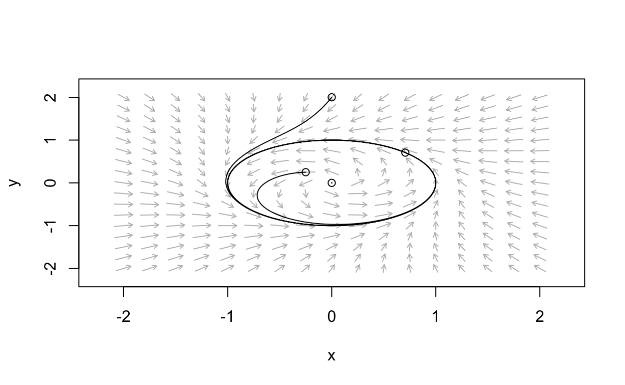
Thus, we see that for this system, trajectories will spiral counterclockwise at a constant rate. Further, trajectories will spiral away from \((0,0)\) and toward the circle \(r=1\) if \(0<r<1\), will orbit around \((0,0)\) on the circle \(r=1\) whenever the initial condition falls on \(r=1\), and spiral toward the circle \(r=1\) whenever \(r > 1\).
We can conclude that the system
\[ \begin{align} \frac{dx}{dt}&=x(1-x^2-y^2) - y \\ \frac{dy}{dt}&=y(1-x^2-y^2) + x \end{align} \]
possesses a limit cycle which corresponds to the unit circle \(r=1\). Further, this limit cycle is stable since any trajectory that begins off of \(r=1\) will eventually approach \(r=1\). Limit cycles may also be unstable as we will see shortly.
Here is a phase portrait for the system obtained using
phaseR.

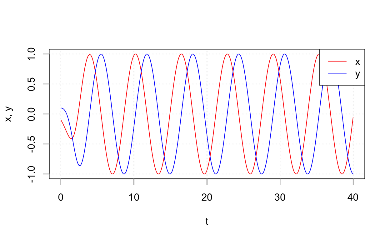
Let’s also plot a times-series for this system.

Obviously, the system has a periodic solution.
Question: What can you say about the phase portrait for a system that takes the following form when written in terms of polar coordinates?
\[ \begin{align} \frac{dr}{dt} &= r(r^2 - 1)\\ \frac{d\theta}{dt} &= 1 \end{align} \]
What about this system?
\[ \begin{align} \frac{dr}{dt} &= r(1 - r)(r - 2)\\ \frac{d\theta}{dt} &= 2 \end{align} \]
Analyzing Limit Cycles
Given an autonomous system
\[ \begin{align} \frac{dx}{dt} &= f(x,y) \\ \frac{dy}{dt} &= g(x,y) \end{align} \] we can always convert to an equivalent system in polar coordinates with the form
\[ \begin{align} \frac{dr}{dt} &= \tilde{f}(r,\theta) \\ \frac{d\theta}{dt} &= \tilde{g}(r,\theta) \end{align} \]
but in general, we can not always decouple the two equations as we were able to do with our previous example system. So how do we analyze systems that may possess a limit cycle? First off, note that linearization does not explicitly detect limit cycles. Nevertheless, it is useful to begin an analysis by finding equilibrium values and the linearization of the system at the equilibria. Next, convert the system to polar coordinates and try to see if this is helpful. If not, then we need to consider other techniques. Namely, we might be able to rule out the possibility of there being any closed trajectories. We will discuss techniques for this in the next set of notes. If you can not rule out closed orbits, then the so-called Poincarè-Bendixson theorem can often be used to derive the existence of a limit cycle. We will cover as well in a later section of notes.
Summary
We have introduced the notion of limit cycle for a two-dimensional nonlinear autonomous system. Further, we have indicated how limit cycles correspond to a periodic solution of a system. In the next set of notes, we will study additional techniques that can be used to determine if a system may possess a limit cycle or not. After we study these techniques, we will see some systems relevant in biomathematics that do possess limit cycles.
Further Reading
See Chapter 7 from (Strogatz 2015) for more on limit cycles.